Carlos Pestana Barros & Nicolas Peypoch
A Comparative Analysis of Productivity Change in Italian and Portuguese Airports
WP 006/2007/DE _________________________________________________________
João Carlos Lopes & Tânya Araujo
The economic performance of Portuguese and
Spanish regions: A network dynamics
approach
WP 04/2012/DE/UECE _________________________________________________________
De pa rtme nt o f Ec o no mic s
W
ORKINGP
APERS ISSN Nº 0874-4548The economic performance of Portuguese and Spanish
regions: A network dynamics approach
João Carlos Lopes* and Tanya Araújo
ISEG - School of Economics and Management, Technical University of Lisbon,
and UECE - Research Unit on Complexity and Economics
Abstract. This paper contributes to further understanding the economic performance of Portuguese and Spanish regions, using a stochastic network approach. The empirical analysis is made at the territorial level of NUT 3 regions and covers the period 1995-2008. The performance of regions is based on GDP per capita at Purchasing Power Standards. The network analysis is based on a metric space built from the correlation coefficients between the log-difference of annual growth rates. The metric space and the corresponding topological coefficients are compared with the independent performance of randomly generated data. The metric space is graphically represented along the 3 dominant eigenvalues and the strongest connections are selected and represented in a network of Iberian regions. The main purpose of this research is to find the most relevant geographical and demographic determinants of regional development, namely a “border effect”, an “interiority (without border) effect”, a “coastal effect”, a “metropolitan effect” and an “ultra periphery effect”.
* Corresponding author:
e-mail:[email protected]
Full address:
Prof. João Carlos Lopes ISEG - UECE
1. Introduction
This paper deals with the economic performance of Portuguese and Spanish regions at NUTS 3 level, in the time period 1995-2008. After a long history of division, conflicts, misunderstanding and weak economic relations, the two Iberian countries started a period of partnership and strong economic integration in 1986, after both becoming members of the European Economic Communities, now European Union. A thorough analysis of the changes in economic relationships between Portugal and Spain before and after European integration is made in Diéguez and Caramelo (2001). According to these authors, one of the main repercussions of this political event was felt in the common border areas of these countries, that finally started to cooperate, after centuries of hostility, or mutual ignorance at best. However, they recognize that it is far from exhausted the full potential of economic cooperation between these regions, which is corroborated in Carvalho and Mourato (2010), that call attention to the weak interregional commercial flows in cause. This result is not unexpected, as McCallum (1995) has already taken a similar conclusion, when assessing the importance of national borders to Canadian-US regional trade patterns.
The main purpose of this paper is to empirically quantify the strength (or weakness) of a “border effect” in the dynamics of regional performance in the Iberian Peninsula, at the NUTS 3 level. In accomplishing this task, we also try to measure geographic and demographic effects, dividing the remaining regions (those not around the common border between Portugal and Spain) in “coastal” and “interior” (a self explained division) and large “metropolitan” ones (those with urban areas with a population of more than 700.000 persons in Spain, and more than 300.000 in Portugal). Initially, we also isolated the two capital regions (Lisbon and Madrid) but the preliminary results proved to be ineffective this further division.
dynamics. Using a metric related the correlation coefficients between the GDP per capita if the Iberian regions, a method is applied to reconstruct a metric space from empirical data. Having a metric defined in the space of regions, network topological coefficients are used to extract further information from the data, namely illustrating the relative strength of the administrative, geographic and demographic effects on the regional development process. Section 5 ends the paper with some concluding remarks.
2. Data and classification of regions
The data for the empirical results of this work is based on the values of GDP per head at purchasing power standards for the regions of Portugal and Spain, at the NUTS 3 level, and were obtained from the Regional Database of EUROSTAT: Regional Economic Accounts (available at: http://ec.europa.eu/eurostat ). For the details about this database see EUROSTAT (2010).
The period covered is 1995-2008, but in some exercises we divide this period in two phases: 1995-2001 and 2001-2008, namely when we are searching for the top and bottom economic growth regions. Particularly in Portugal, there is a clear change in global and (therefore) regional economic performance between the 1990’s and the following decade, as will be clear in the next section. In Spain, this change in economic growth momentum occurred much later, and it was not practically felt until 2008 (only after the global macroeconomic crisis of 2009).
The regional level at which the analysis of this paper is made is NUTS 3, because it is preferable to assess the regional economic performance at the most detailed level as possible, and the NUTS 2 level is not adequate for this purpose.
The next step is to classify the regions according to our analytical purpose. As we give priority to assessing the (political and administrative) effect on regional growth performance of the existence of a common border, we begin by isolating the 17 regions affected by this criterion (10 in Portugal and 7 in Spain), and call them (common) “Frontier” regions.
The next criterion was of a pure geographical nature, dividing the regions in those having some part of its territory with a see cost (“Coastal” regions) and those having not (“Interior” regions). This is an obvious classification that does not deserve much explanation. However, we complement this classification with a further criterion, a demographic one due to the agglomeration economies associated to the literature on the new economic geography (Krugman, 1991; Krugmam and Venables, 1995) and endogenous growth (Lucas, 1988). A autonomous category is created for large “Metropolitan” regions, being considered (relatively) large those having more than 700.000 inhabitants in Spain and more than 300.000 in Portugal (but we admit that a low separating level may be considered and tested). Combining both criteria we have then 38 (non common frontier) interior regions (10 in Portugal; 28 in Spain), 22 (non common frontier) coastal regions (6 in Portugal; 16 in Spain) and 12 large metropolitan regions (3 in Portugal; 9 in Spain).
Finally, being particularly different, for political, administrative and geographical reasons, we group in a separated category the so called (ultra-)”Peripheral” regions of Madeira, Azores, Baleares, Canarias, Ceuta and Melilla.
A list with all the regions considered, the corresponding NUTS 3 code and the classification label (with the first letter, P or E, meaning the country, and the second letter, F, C, I, M or P, corresponding to the above regional definitions) is presented in Appendix 1.
3. Regional economic growth and convergence
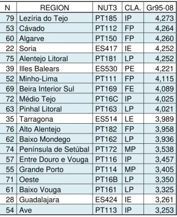
Portuguese regions representing the most part of the 20 bottom growth cases (Table 3.2).
< Take in Table 3.1 > < Take in Table 3.2 >
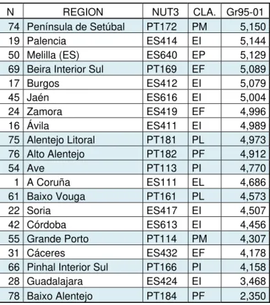
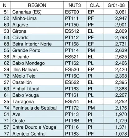
However, this global picture hides an important change in individual growth experiences, with a significant deterioration of regional (and of course, national) growth conditions in Portugal between the sub-periods 1995-2001 (Table 3.3 and 3.4) and 2001-2008 (Tables 3.5 and 3.6), giving rise to what many Portuguese economists now call the “lost decade”. On the other side and as it is also well known, in Spain this deterioration in growth momentum appears much later, and is not seen in these results.
< Take in Table 3.3 > < Take in Table 3.4 > < Take in Table 3.5 > < Take in Table 3.6 >
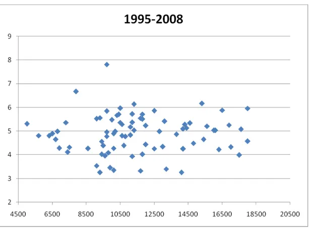
As most of Portuguese regions start from low levels of economic development, it comes with no surprise the apparent lack of real convergence in this period, in the context of all the Iberian regions, both in the sigma version, measured by the coefficient of variation of GDP per capita (Figure 3.1), as in the beta kind of convergence (Figure 3.2), given by the absence of negative correlation between annual average growth and initial level of GDP per capita (for a technical description of these notions of convergence, and many empirical examples, see Barro and Sala-i-Martin, 2005).
The other effects to be assessed in this empirical paper, administrative (border), geographical (coastal versus interior, or peripheral) or demographic (metropolitan areas) appear not to be determinant in the growth process of NUTS 3 regions. All these examples punctuate the (relative) growth successes and low performance cases (not really un-successes, as there are rare examples of negative average regional growth in this period).
And so, in order to better understand the strength of these factors in the regional growth dynamics of Portuguese and Spanish regions, the next section describes the application of a network approach.
4. Iberian regional performance through a network approach
Using a stochastic geometry technique over the time evolution of the GDP per head values of a set of Portuguese and Spanish regions, it is possible to identify a geometric structure which is conveniently described by a network approach.
The stochastic geometry technique is simply stated in the following terms:
1) pick a set of N regions and their historical data over a chosen time interval and 2) considering the vectors p(k)with the GDP per head yearly values of each region
(k), define a normalized vector
2 2 ) ( ) ( ) ( ) ( ) ( k p k p n k p k p k (1)
where n is the number of components (number of time labels) in the vector p and < > the average value of the observations over time,
3) compute an Euclidian distance (dk,l) between each pair of regions ) ( ) ( ) 1 ( 2
, C k l
dkl kl
(2) where Ckl is the correlation coefficient between the pair of regions (k and l)
computed along the chosen time interval (of length n).
correlations between regions is small, then the corresponding manifold will be a low-dimensional entity.
The following stochastic geometry technique was used for this purpose.
1) after the distances (dk,l) are calculated for the set of N regions, they are embedded in RN-1 with coordinatesx(k).
2) the center of mass R is then computed and the coordinates reduced to the center of mass
k k x R
k ( ) (3) R k x k
y( ) ( ) (4) 3) the matrix
) ( ) (k y k y T j k i ij
(5)is diagonalized to obtain the set of normalized eigenvalues and eigenvectors
i,ei
. 4) the eigenvectors eidefine the characteristic directions of the set of regions and theircoordinates )zi(k are obtained by the projection i i i k y e z ( )
(6)
5) the characteristic directions correspond to the eigenvalues (i) that are clearly different from those obtained from surrogate data. They define a reduced subspace of dimension d, which carries the systematic information related to the correlation structure of the regional space.
This corresponds to the identification of empirically constructed variables that drive the set of regions, and, in this framework, the number of surviving eigenvalues is the effective characteristic dimension of this regional space.
In this paper we apply such a dimensional reduction for the identification of strongly and weakly correlated regions, accordingly to the simultaneous evolution of their GDP per capita values along a certain time interval.
4.1 From a geometrical to a topological approach
The existence of a distance metric allows for the application of a topological approach in order to identify a network of regions associated to the low-dimensional regional space. From the matrix of distances dk,l computed in the reduced d-dimensional space, we apply the hierarchical clustering process to construct the minimal spanning tree (MST) that connects the N regions. Then the Boolean graph B is defined by setting
otherwise l
k b
L l k d if l
k b
0 ) , (
) , ( 1
) , (
(7) where Lis the smallest threshold distance value that assures connectivity of the whole network in the hierarchical clustering process.
4.2 Regional spaces and their corresponding networks of regions
Results were computed using actual data, which consists in the set of yearly GDP per capita values of 81 regions with a time window of 13 years, from 1995 to 2008. We
also compute results from surrogate data, i.e. data generated by permuting the GDP per capita values of each region randomly in time. As each region is independently
permuted, time correlations among regions disappear, while the resulting surrogate data preserve the mean and the variance that characterize actual data.
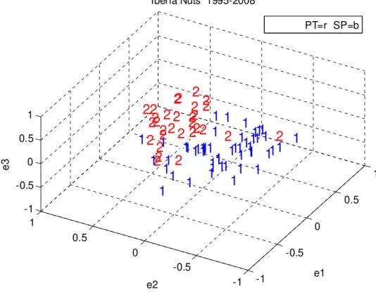
Comparing results obtained from actual data with results computed from surrogate data has shown that the regional space has only three dimensions (the corresponding manifold can be contained in a 3-dimensional space). Figure 4.1 shows the projection of the coordinates of the set of 81 regions on these three characteristic directions.
< Take in Figure 4.1 >
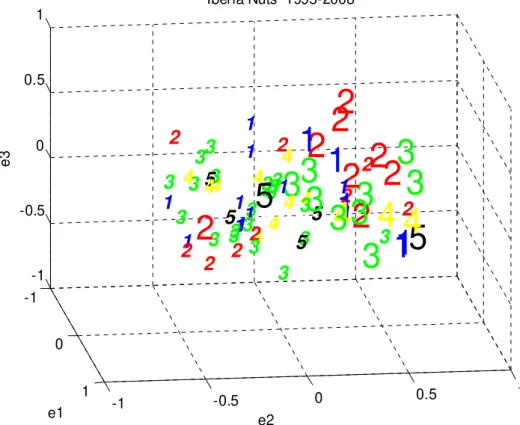
In the 3-dimensional space presented in Figure 4.2, the 81 Portuguese and Spanish regions are represented according to the geographical and demographic classification described in section 2, according to the following legend: 1:Coastal, 2:Border, 3:Interior, 4:Metropolitan, 5:Peripheral. When the region is a Portuguese one it is represented in large, while Spanish regions have a smaller representation. Again, the observation of the 3-dimensional space of regions seems to lead to the identification of a tendency towards the occupation of different space slots depending on the country: Portuguese regions seem to be concentrated in the right side of the plot while the Spanish ones are mostly in the left. Moreover, the Interior regions seem to spread all over the 3-dimensional space, while the Border regions are slightly less uniformly distributed on this space.
< Take in Figure 4.2 >
When the geometric distances computed in the reduced 3-dimensinal space are used to define the projected Boolean graph B (as in Equation 7), it was empirically found that the set of 81 regions correspond to a highly connected network (the network degree is around N/2) where the lack of sparseness makes unadvised the computation of typical topological coefficients as clustering and path length.
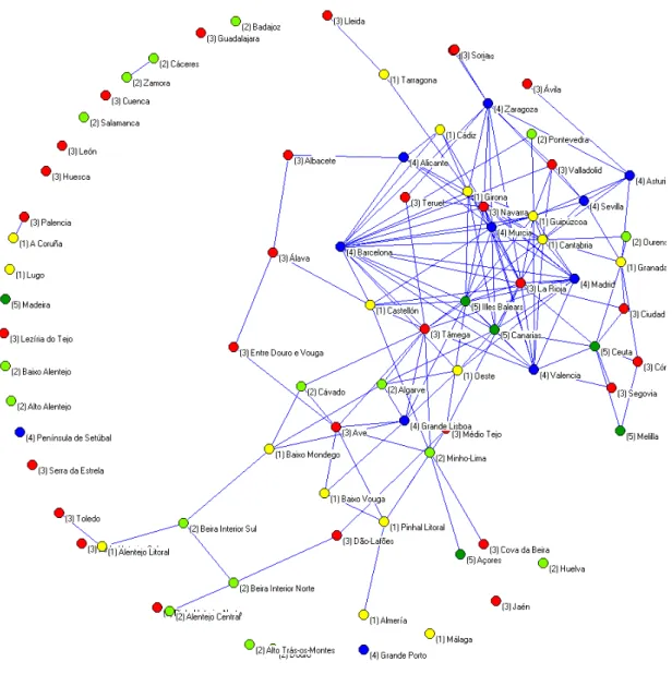
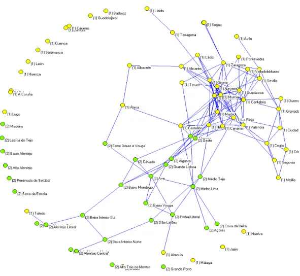
Due to the same reason, in graphically representing the derived network of regions we opt to sort the whole set of distances in ascending order and to exclude the links between regions whose distance occupy a ranking position greater than 2N in the sorted list. In so doing, the degree of the network equals 2 and overloading the graph with a huge amount of links is avoided, allowing for the observation of some linkage patterns as the images in figures 4.3, 4.4 and 4.5 show. These three images present the same network under different drawing options (Pajek was used as the drawing tool).
< Take in Figure 4.3 > < Take in Figure 4.4 >
group of Metropolitan regions is the most strongly correlated one. Its degree of linkage is high either considering the links with regions that are inside or outside the Metropolitan group. Conversely, the Interior and the Border groups are very weakly connected ones.
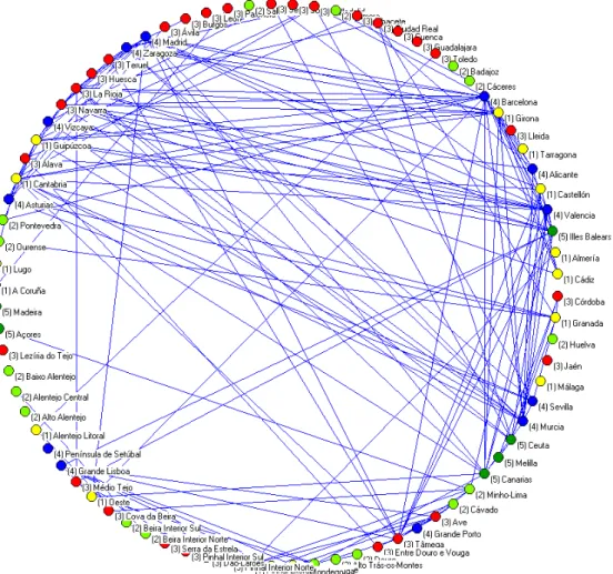
The drawing option adopted in Figure 4.5 allows for the observation that Spanish regions are more connected than the Portuguese ones, showing that country matters when links are defined as function of the correlation between regions performance. This result confirms the findings obtained when assessing the growth and convergence dynamics of the Iberia Peninsula regions (section 3).
< Take in Figure 4.5 >
Another interesting result is that not only Spanish regions are more connected than the Portuguese ones but also that they tend to be strongly correlated with their national counterparts than with the Portuguese regions, independently of how similar are them in terms of their corresponding regional classification.
5. Concluding remarks
In this paper an empirical study of the economic performance of Portuguese and Spanish regions is made, using a traditional growth and convergence analysis and a stochastic network approach.
The study is conducted at the territorial level of NUT 3 regions and covers the period 1995-2008. The economic performance of regions is based on GDP per head at Purchasing Power Standards and the data was obtained from the Regional Accounts available for free at the site of Eurostat.
Besides the obvious criterion of country belonging, a classification was made based on geographical and demographic caractheristics, being the regions divided in Interior, Coastal, (common-) Border, Metropolitan and Peripheral, in order to test if these caractheristics have significant growth effects.
Spanish regions generally overcoming Portuguese ones) and the apparent absence of clear geographic or demographic effects (with a diversified group of regions, both in “winners” and “(relative) loosers” groups. Consistent with the described “country effect”, the results point to an absence of both of the so-called sigma and beta regional convergence, when we use all the Iberian Peninsula regions as the reference set.
The network analysis was based on a metric space built from the correlation coefficients between the log-difference of annual growth rates. The metric space and the corresponding topological coefficients were compared with the independent performance of randomly generated data. The metric space is graphically represented along the 3 dominant eigenvalues and the strongest connections are selected and represented in a network of Iberian regions. Our main results showed the presence of a “metropolitan effect” on regional GDP per head dynamics.
A further step of this research will be to assess the network dynamics of economic (GDP) and demographic (population) evolutions that support the trends studied thus far.
Acknowledgements. Financial support by FCT (Fundação para a Ciência e a Tecnologia), Portugal is gratefully acknowledged.
References
Araújo, T. and Louçã, F. (2007), The Geometry of Crashes - A Measure of the Dynamics of Stock Market Crises, Quantitative Finance 7, 63-74.
Araújo, T. and Louçã, F. (2008) The Seismography of Crashes in Financial Markets, Physics Letters A 372, 429-434.
Barro, R. and Sala-i-Martin, X. (2005), Economic Growth, McGraw-Hill, New York. Carvalho, R. and Mourato, J. (2010), Border Effect in Interregional Iberian Trade,
Paper presented at the XXXVI Reunión de Estudios Regionales, AECR, Badajoz. Diéguez, V. C. and Caramelo, S. (2001), The evolution of the Spanish-Portuguese
border process of European integration, Paper presented at the 41st Congress of the European Regional Science Association, Zagreb.
Krugman, P. (1991), Geography and trade, London: MIT Press/Leuven.
Krugmam, P. and Venables, A. (1995), Globalization and the inequality of nations, Quarterly Journal of Economics 110 (4), 857-880.
Lopes, J.C., Araújo, T., Dias, J. and Amaral, J.F. (2011), National Industry Clusters and the Structure of Industry Output Dynamics: a Stochastic Geometry Approach, Portuguese Journal of Quantitative Methods, forthcoming.
Lucas, R. (1988), On the Mechanics of Economic Development, Journal of Monetary Economics 22 (1988) 3-42.
McCallum, J. (1995), "National borders matter: Canadian-US regional trade patterns, American Economic Review 85, 615-623
Tables:
Table 3.1 Top 20 growth regions: 1995-2008
N REGION NUT3 CLA. Gr95-08
81 Madeira (PT) PT300 PP 7,815
30 Badajoz ES431 EB 6,675
9 Vizcaya ES213 EL 6,165
49 Ceuta (ES) ES630 EP 6,134
4 Pontevedra ES114 EB 5,965
7 Álava ES211 EI 5,959
8 Guipúzcoa ES212 EC 5,885
6 Cantabria ES130 EC 5,858
41 Cádiz ES612 EC 5,845
40 Almería ES611 EC 5,727
5 Asturias ES120 EC 5,714
44 Huelva ES615 EB 5,708
24 Zamora ES419 EB 5,671
43 Granada ES614 EC 5,563
1 A Coruña ES111 EC 5,546
80 Açores (PT) PT200 PP 5,521
18 León ES413 EI 5,511
46 Málaga ES617 EC 5,477
19 Palencia ES414 EI 5,414
16 Ávila ES411 EI 5,367
Table 3.2 Bottom 20 growth regions: 1995-2008
N REGION NUT3 CLA. Gr95-08
79 Lezíria do Tejo PT185 IP 4,273
53 Cávado PT112 FP 4,264
60 Algarve PT150 FP 4,260
22 Soria ES417 IE 4,252
75 Alentejo Litoral PT181 LP 4,252
39 Illes Balears ES530 PE 4,221
52 Minho-Lima PT111 FP 4,115
69 Beira Interior Sul PT169 FE 4,089
72 Médio Tejo PT16C IP 4,025
63 Pinhal Litoral PT163 LP 4,021
35 Tarragona ES514 LE 3,989
76 Alto Alentejo PT182 FP 3,958
62 Baixo Mondego PT162 LP 3,936
74 Península de Setúbal PT172 MP 3,538 57 Entre Douro e Vouga PT116 IP 3,457
55 Grande Porto PT114 MP 3,405
71 Oeste PT16B LP 3,350
61 Baixo Vouga PT161 LP 3,325
28 Guadalajara ES424 IE 3,261
Table 3.3 Top 20 growth regions: 1995-2001
N REGION NUT3 CLA. Gr95-01
81 Madeira (PT) PT300 PP 9,586
40 Almería ES611 EL 8,428
77 Alentejo Central PT183 PF 8,384
30 Badajoz ES431 EF 7,803
65 Dão-Lafões PT165 PI 7,712
68 Beira Interior Norte PT168 EF 7,679
80 Açores (PT) PT200 PP 7,186
8 Guipúzcoa ES212 EL 7,099
34 Lleida ES513 EI 7,065
41 Cádiz ES612 EL 7,053
37 Castellón ES522 EL 6,991
7 Álava ES211 EI 6,859
15 Madrid ES300 EM 6,856
6 Cantabria ES130 EL 6,752
46 Málaga ES617 EL 6,752
67 Serra da Estrela PT167 PI 6,752
48 Murcia ES620 EL 6,613
36 Alicante ES521 EL 6,591
44 Huelva ES615 EF 6,529
38 Valencia ES523 EL 6,522
Table 3.4 Bottom 20 growth regions: 1995-2001
N REGION NUT3 CLA. Gr95-01
74 Península de Setúbal PT172 PM 5,150
19 Palencia ES414 EI 5,144
50 Melilla (ES) ES640 EP 5,129
69 Beira Interior Sul PT169 EF 5,089
17 Burgos ES412 EI 5,079
45 Jaén ES616 EI 5,004
24 Zamora ES419 EF 4,996
16 Ávila ES411 EI 4,989
75 Alentejo Litoral PT181 PL 4,973
76 Alto Alentejo PT182 PF 4,912
54 Ave PT113 PI 4,770
1 A Coruña ES111 EL 4,686
61 Baixo Vouga PT161 PL 4,573
22 Soria ES417 EI 4,507
42 Córdoba ES613 EI 4,456
55 Grande Porto PT114 PM 4,307
31 Cáceres ES432 EF 4,178
66 Pinhal Interior Sul PT166 PI 4,158
28 Guadalajara ES424 EI 3,468
Table 3.5 Top 20 growth regions: 2001-2008
N REGION NUT3 CLA. Gr01-08
81 Madeira (PT) PT300 PP 6,320
1 A Coruña ES111 EL 6,288
24 Zamora ES419 EF 6,254
78 Baixo Alentejo PT184 PF 6,167
49 Ceuta (ES) ES630 EP 5,902
9 Vizcaya ES213 EL 5,895
5 Asturias ES120 EL 5,870
18 León ES413 EI 5,773
30 Badajoz ES431 EF 5,718
16 Ávila ES411 EI 5,692
19 Palencia ES414 EI 5,647
31 Cáceres ES432 EF 5,635
66 Pinhal Interior Sul PT166 PI 5,533
4 Pontevedra ES114 EF 5,529
43 Granada ES614 EL 5,528
50 Melilla (ES) ES640 EP 5,329
17 Burgos ES412 EI 5,327
2 Lugo ES112 EL 5,217
7 Álava ES211 EI 5,194
Table 3.6 Bottom 20 growth regions: 2001-2008
N REGION NUT3 CLA. Gr01-08
51 Canarias (ES) ES700 EP 3,061
52 Minho-Lima PT111 PF 2,947
60 Algarve PT150 PF 2,901
33 Girona ES512 EL 2,809
53 Cávado PT112 PF 2,798
68 Beira Interior Norte PT168 EF 2,731
55 Grande Porto PT114 PM 2,639
36 Alicante ES521 EL 2,625
62 Baixo Mondego PT162 PL 2,466
39 Illes Balears ES530 EP 2,420
72 Médio Tejo PT16C PI 2,398
37 Castellón ES522 EL 2,395
63 Pinhal Litoral PT163 PL 2,388
61 Baixo Vouga PT161 PL 2,267
35 Tarragona ES514 EL 2,252
74 Península de Setúbal PT172 PM 2,176
54 Ave PT113 PI 1,970
71 Oeste PT16B PL 1,779
57 Entre Douro e Vouga PT116 PI 1,371
Figures:
Figure 3.1: Sigma (non-)convergence: GDPpc – coefficient of variation
Figure 4.1: Projection of the 81 regions’ coordinates on the 3 characteristic directions -1 -0.5 0 0.5 1 -1 -0.5 0 0.5 1 -1 -0.5 0 0.5 1 e1 1 1 2 1 1 1 1 1 1 1 1 1 1 1 1 1 1 1 1 1 1 1 1 1 2 1 1 1 11 1 1 11 1 1
Iberia Nuts 1995-2008
22 1 11 11 2 1 2 2 1 2 2 2 2 2 1 1 1 2 2 2 2 2 1 2 1 2 1 1 22 1 e2 2 2 2 2 2 1 2 2 2 2 1 e3
PT=r SP=b
Figure 4.2: Projection by kind of (geographic and demographic) region
-1
0
1
-1 -0.5 0 0.5 1
-1 -0.5 0 0.5 1
5
3
4
23
1
1
2
34
2
3
23
2
3
2
2 1 12
1
4
2
3
1
52
3
3
4 31
3 53
4 4Iberia Nuts 1995-2008
3 1 2 3 3 4 3 3 3 e2
5
4 4 2 3 3 1 1 1 3 1 1 1 2 3 3 5 4 3 3 3 5 2 42
3 3 4 1 2 3 2 3 1 e1 e3Legend: 1: Coastal (blue), 2: Border (red), 3: Interior (green), 4: Metropolitan (yellow), 5: Peripheral (black);
Figure 4.3: The network of regions: geographical and demographic effects (strongest 162 (2N) links)
Figure 4.5: The network of Regions: country effect
Legend:
Appendix 1: Portuguese and Spanish NUTS 3 level regions and classification (cont.)
N REGION NUT3 CLA.
42 Córdoba ES613 EI
43 Granada ES614 EL
44 Huelva ES615 EF
45 Jaén ES616 EI
46 Málaga ES617 EM
47 Sevilla ES618 EM
48 Murcia ES620 EL
49 Ceuta (ES) ES630 EP
50 Melilla (ES) ES640 EP
51 Canarias (ES) ES700 EP
52 Minho-Lima PT111 PF
53 Cávado PT112 PF
54 Ave PT113 PI
55 Grande Porto PT114 PM
56 Tâmega PT115 PI
57 Entre Douro e Vouga PT116 PI
58 Douro PT117 PF
59 Alto Trás-os-Montes PT118 PF
60 Algarve PT150 PF
61 Baixo Vouga PT161 PL
62 Baixo Mondego PT162 PL
63 Pinhal Litoral PT163 PL
64 Pinhal Interior Norte PT164 PI
65 Dão-Lafões PT165 PI
66 Pinhal Interior Sul PT166 PI
67 Serra da Estrela PT167 PI
68 Beira Interior Norte PT168 PF
69 Beira Interior Sul PT169 PF
70 Cova da Beira PT16A PI
71 Oeste PT16B PL
72 Médio Tejo PT16C PI
73 Grande Lisboa PT171 PM
74 Península de Setúbal PT172 PM
75 Alentejo Litoral PT181 PL
76 Alto Alentejo PT182 PF
77 Alentejo Central PT183 PF
78 Baixo Alentejo PT184 PF
79 Lezíria do Tejo PT185 PI
80 Açores (PT) PT200 PP