M
ASTER IN
F
INANCE
M
ASTERS
F
INAL
W
ORK
D
ISSERTATION
T
HE DETERMINANTS OF CORPORATE CAPITAL
STRUCTURE
:
EVIDENCE FROM
P
ORTUGUESE LISTED
COMPANIES
,
1984-1988
M
ARTA DAS
N
EVES
R
AMOS
H
IPÓLITO
M
ASTER IN
F
INANCE
M
ASTERS
F
INAL
W
ORK
D
ISSERTATION
T
HE DETERMINANTS OF CORPORATE CAPITAL
STRUCTURE
:
EVIDENCE FROM
P
ORTUGUESE LISTED
COMPANIES
,
1984-1988
M
ARTA DAS
N
EVES
R
AMOS
H
IPÓLITO
G
UIDANCE
:
P
EDRO
J
OSÉ
M
ARTO
N
EVES
My special thanks to my supervisor Professor Pedro José Marto Neves, whose
achievement of this work would not be possible without his knowledge and complete
availability.
To my family for unconditional love.
To my boyfriend Hugo for the love, support and understanding.
Finally, I want to express my gratitude to my parents by dedicating this thesis to them.
In honour of my work and the person that you help me becoming, I thank you for all
that you taught me, for believing and supporting me along the different stages of my
O propósito desta tese é analisar a estrutura de capital de empresas portuguesas cotadas
em bolsa, focando na relação entre o nível de endividamento e os fatores determinantes
considerados mais relevantes na literatura financeira. A amostra utilizada neste estudo
empírico é composta por 87 empresas cotadas, tendo sido recolhida informação
contabilística referente ao período de 1984 a 1988. Com base numa análise de dados em
painel, os resultados obtidos sugerem que a dimensão e a estrutura do ativo são fatores
determinantes do endividamento. Os resultados contribuem para complementar a
informação disponibilizada em estudos existentes, e para providenciar um conhecimento
mais profundo acerca das decisões que as empresas tomam para a sua estrutura de
capitais.
This dissertation aims to analyze the capital structure of Portuguese listed companies on
the stock market, focusing on the relationship between the level of debt and its most
relevant determinant factors considered in financial literature. The sample used in this
empirical study consists of 87 listed companies and accounting information has been
collected for the period 1984-1988. Using a panel data approach, we found that size and
asset tangibility are determinant factors of the debt level. The results contribute to fill a
gap on Portuguese history, helping to complement existing studies and to provide a
deeper understanding of the companies’ decisions about their capital structure.
Acknowledgments ... iii
Resumo ... iv
Abstract ... v
1. Introduction ... 1
2. Theoretical Framework and Research Hypotheses ... 3
2.1. Traditional Theory ... 3
2.2. Modigliani & Miller ... 3
2.3. Trade-off Theory ... 6
2.4. Pecking Order Theory ... 9
2.5. Research Hypothesis ... 10
3. Database and Methodology ... 15
3.1. Sample ... 15
3.2. Variables ... 17
3.2.1. Dependent Variables ... 17
3.2.2. Independent Variables ... 18
3.3. Methodology ... 19
3.4. The Models ... 20
4. Discussion of Empirical Results ... 23
5. Conclusions ... 27
References... 29
Table I - Theories Expected Relations ………..…….………10
Table II - Sample Distribution by Industry …….………...16
Table III - Proxies of the dependent variable ……….…....…18
Table IV - Proxies of the independent variables………...19
Table V - Expected and Observed Relations in the Regression Models………...…..…26
Table a.1 - List of Companies……….…………34 Table a.2 - Correlation Matrix……….37
Table a.3 - Summary of Descriptive Statistics ……….………..38 Table a.4 - Results of Y1regression model……….………..……..39
Table a.5 - Results of Y2regression model……….………...….40
Table a.6 - Results of Y3regression model……….………....41
List of Figures
Figure 1 - Sample Distribution by Industry (%)………..…….………...………...16Figure 2 - Evolution of listed firms on the Portuguese Stock Market ………...17
1.
Introduction
Firms' capital structure has been a controversial and widely discussed subject in
academic literature of Finance. Setting a financing policy that maximizes the value of
the assets of a company is crucial to its profitability and sustainability along its lifespan.
Several empirical studies have been conducted worldwide in order to identify the factors
that better explain the way businesses are financed and predict their results through
different models. However, the heterogeneity of results on empirical evidence suggests
that this issue has not been completely addressed.
Companies have two main sources of funding their business activity: through equity or
debt. Firms can find much of their financing needs internally, using only the owner’s
equity to run the company. Nevertheless, some of them will naturally feel the need for
debt or a mix of internal and external sources to be able to invest in new projects or
long-term assets.
There are several empirical studies about the capital structure decisions of Portuguese
firms (for instance: Antão & Bonfim, 2008; Serrasqueiro & Rogão, 2009; Vieira, 2013).
However, these works focus mainly in the period after 1990. Only a recent work
(Gonçalves, 2015) studies the capital structure of the large Portuguese manufacturing
firms in the eighties. With the present work, we aim to continue this effort focusing on
other group of firms: the firms listed on the stock markets.
The second half of the 1980 decade was an interesting period regarding capital markets
in Portugal. After the Carnation Revolution of 1974 and the nationalization process that
operations were suspended on April 24, 1974 and the market only reopened on January
12, 1976 for Treasury bonds and on March 7, 1977 for other securities. Still, the
number, dimension and diversity of private firms with their assets quoted on the
exchange were then very small (Costa & Mata, 2011). During the eighties, particularly
in the second half of the decade, there was a huge increase in the number of companies
present on the stock market and its volume of transactions has grown exponentially
(Gomes et al, 1987). Those companies are our object of study.
By examine the decisions about the capital structure of listed companies, we will assess
to what extend the borrowing decisions of those firms follow the theoretical
relationships stated by the financial literature. We will focus on the relationship between
debt level and the most relevant determinants suggested in the literature, namely: size,
growth, profitability, assets composition, non-debt tax shields and business risk.
The work is organized as follows. Section 2 reviews the related literature and presents
our hypotheses. Section 3 describes the data and methodology used in testing them.
2.
Theoretical Framework and Research Hypotheses
In this section we present the literature review and corresponding hypothesis for
investigation concerning debt and its determinant factors in the choice of the capital
structure, according to the most relevant theories.
2.1.Traditional Theory
The traditionalist approach of Durand (1952) defends the existence of an optimal capital
structure that maximizes the value of a company and minimizes its cost of capital.
According to the author, the cost of capital remains stable up to a certain level of
indebtedness, from which it begins to increase towards an increment in the bankruptcy
risk.
In particular, a company should indebted up until the weighted average cost of capital
(WACC) reaches its minimum, since this point represents the optimal value of the
company’s capital structure, and hence its maximum value.
2.2.Modigliani & Miller
In 1958, Modigliani & Miller's article "The Cost of Capital, Corporate Finance and
Theory of Investment" originated the modern financial theory with the capital structure
irrelevance proposition, based on a perfect capital market world and the law of one
price. This pioneering study states that the market value of a company is independent of
its capital structure, being mainly defined by its investment decisions.
Rational behavior of investors;
The company issues two types of financial securities: debt without risk (bonds)
and equity (shares);
Investors have homogenous expectations about future profitability;
Companies are grouped into classes of "equivalent income", which means the
shares of several companies are in homogeneous groups and are perfectly
substitutable for each other.
MM's presented two proposals to demonstrate the irrelevance of the capital structure on
a firm’s value. In Proposition I, on the absence of taxes or other transaction costs, the
total cash flow paid out to all security holders of a firm equals the total cash flow
generated by the firm’s assets. Thus, by the Law of One Price, it is irrelevant if the
assets were originate by internal or external capital, since the value of the firm depends
exclusively on the ability of its assets to generate value and growth opportunities. If
these factors are constant, so it will be its value, being independent of the type of
financing. Additionally, the weighted average cost of capital of the company is constant
among companies belonging to the same risk class.
This model has also an arbitration adjustment mechanism, when the expected return on
similar assets of two companies differ regarding its equilibrium value, investors will
notice an arbitrage opportunity and start a process of selling the shares of the overvalued
company and buy the shares of the undervalued company. This process is repeated until
the companies had expected profitability identical within the same class or until the
In Proposition II, it was shown that the rate of return that investors expect to receive
depends on the equity ratio. The authors concluded that the expected yield on ordinary
shares of an indebted company increases proportionally with the equity ratio, estimated
at market values.
Later on, Modigliani & Miller (1963) realizing the limitations of their initial study,
published a new article "Corporate Income Taxes and the Cost of Capital: A
Correction", where they already considered the tax effect on the company's decision in
its capital structure.
MM recognized that with taxes, the first proposition of irrelevance would not be the
most appropriate one, since companies have an advantage using debt instead of internal
sources due to the benefit of debt tax shields, allowing the deduction of financing costs.
As a result of the leverage effect, originated by the arbitration adjustment mechanism
predicted in Proposition I, the expected return of shares in a company within the same
class, on balance, tends to present a similar value. This situation leads to an increase of
wealth for its shareholders. In other words, companies are encouraged to finance
through debt rather than equity, once the higher the value of the assets financed by debt
capital, the greater the value of the company will be. Therefore, there will be an optimal
capital structure able to increase the value of companies and minimize its weighted
average cost of capital.
The correction MM (1963) for the propositions I and II presented in 1958 was based on
the following assumptions:
Absence of transaction costs;
Equality between the interest rate charged on companies and particulars.
In this context, keeping the assumption of belonging to equivalent income classes, MM
demonstrated that the value of an indebted company, after the deduction of taxes, is
equal to the value of a company not indebted, plus the tax benefits associated with the
debt.
As the indebtedness increases, company’s value and shareholders’ wealth also
increased, so the optimal debt policy should be the one in which the company is fully
funded by debt. However, MM found that, despite the tax effect provided by debt
interest, the company should not borrow fully under the risk of losing flexibility
regarding the treasury management and the choice of its financial sources. Market
imperfections are likely to determine the indebtedness, in particular the restrictions
imposed by lenders when extending credit.
Despite the high criticism received by the work of MM, since their propositions are only
valid in a perfect capital market environment, it was the launch to the beginning of the
studies on a subject until that date rarely discussed.
2.3.Trade-off Theory
In 1963, Modigliani and Miller introduced the tax benefit of debt by adding the
corporate income tax to the original irrelevance proposition. The divergent findings on
MM work led the financial literature along that decade to focus on a deeper study of the
effects of debt and how they are related to a target capital structure. New theories
On the light of this theory, there is an optimal capital structure that maximizes the value
of the company, which results from a trade-off between the tax benefits and insolvency
costs associated with the debt. Kraus & Litzenberger (1973), Scott (1977), Kim (1978)
and Myers (1984) developed models of equilibrium between the benefits and costs of
taxes related to debt, namely, taxes, bankruptcy and agency costs. Also Warner (1977),
Haugen & Senbet (1988) and Brennan & Schweartz (1978) introduced the bankruptcy
costs in models to determine the capital structure (Rogão, 2006).
On a scenario of complete capital markets, Kraus & Litzenberger (1973) proved the
optimal capital structure occurs when: “the total value of a levered firm equals the
value of the firm without leverage plus the present value of the tax savings from debt,
less the present value of financial distress costs” (Berk & DeMarzo, 2013). Formally,
the mathematical equation is the following:
(1)
Hence, equation (1) shows that this theory is supported mainly by two concepts, the
advantages and disadvantages of borrowing. On one hand, firms should consider the
benefits of debt, which include the tax deduction of interest costs and the reduction of
agency costs resulting from excess free cash flow, arising from tax savings. On the
other hand, companies have to weigh the costs related to debt, such as bankruptcy costs
that can occur in excessive debt situation. As well as the possibility of arising agency
costs caused by the conflict of interests between shareholders and lenders, including the
expenses incurred by lenders in the supervision of shareholders with the aim of
Scott (1977) based on the assumption of imperfect capital markets and the possibility of
the company goes into bankruptcy, showed the optimal debt level is an increasing
function of the liquidation value of the firm’s assets and the tax rate on income of the
company.
Assuming perfect capital markets, Kim (1978) considered that the optimal capital
structure involves less funding through debt than their debt capacities. The author
concluded that the borrowing capacity is inferior to the totality of capital. Since
managers seek an optimal capital structure, a debt financing lower than one-hundred
percent is required.
Myers (1965) defended that firms adjust the actual debt level toward a target debt ratio,
which means that a company will be in a continuous process of dynamic compensation
replacing debt for equity and vice versa, until it reaches the optimal debt ratio (Ribeiro,
2001). So, when resorting to debt, companies should establish a target debt ratio to
maximize the tax benefit and minimize the risk of going bankrupt. Graham & Harvey
(2001) and Bancel & Mittoo (2004) results show found evidence to support this
trade-off hypothesis for the U.S market and 16 European countries, respectively (Vieira,
2013).
The determinants of capital structure suggested by the trade-off theory are size, asset
2.4.Pecking Order Theory
A different approach to the capital structure issue is the Pecking Order Theory. This
theory does not claim that companies seek for an optimal target debt ratio instead the
level of debt is defined by the financial needs of a firm.
Based on the study of Donaldson (1962), Myers (1984) and Myers & Majluf (1984)
concluded that adverse selection costs strongly influences investment and financing
decisions of a company. These costs result from asymmetric information between
managers and investors. Managers know better investment opportunities than external
investors and have more information about the value of the company.
Under this theory, companies follow a hierarchical order of preferences when selecting
different sources of financing. Firms prefer to use retained earnings as their primary
source of funding, followed by debt and ultimately by equity. When internal cash flows
are not enough to fund capital expenditures, companies will borrow, rather than issue
equity. Equity capital is the least interesting source of financing for companies as it has
underlying higher asymmetric information costs, making the issue more costly when
compared to other sources of funding.
Myers (2001) argues that pecking order theory helps explaining the fact that most
profitable companies are the ones who borrow less, since they have available more
internal resources to finance their investment projects. In contrast, less profitable
companies need to resort to external financing due to insufficient internal generated
cash flows, which can lead to cumulative debt. Thus, this theory suggests a negative
The determinants of capital structure suggested by the pecking order theory are
profitability, growth opportunities, cash-flow and age.
Table I summarizes the expected relations between the level of debt and the determinant
factors according to the theories presented above.
Table I
Theories Expected Relations
Expected Relations Trade-off Pecking Order
Debt and size + +
Debt and growth - +
Debt and profitability + -
Debt and level of tangible assets + + Debt and non-debt tax shields - n.a.
Debt and business risk n.a. n.a.
2.5.Research Hypothesis
i) Size of the Firm
According to the trade-off theory, larger companies opt for more diversified strategies,
are less prone to bankruptcy and can easily access to credit with favourable conditions.
As they provide more guarantees, firms tend to have more debt in its capital structure.
Also, under the pecking order theory, a positive relationship between size and debt is
defended. Larger companies are more diversified, with better reputation in the market
and less information asymmetry costs, and consequently have greater capacity to incur
Authors like Scott (1977), Warner (1977), Rajan & Zingales (1995), Titman & Wessels
(1988), Baker & Wurgler (2002) and Frank & Goyal (2004) found evidence for the
following hypothesis:
H1: Size is positively related to the level of debt of a firm.
ii) Growth Opportunities
Another issue to address is the relationship between the growth level of companies and
their capital structure. Trade-off theory stands for a negative relationship between debt
and growth, stating that companies avoid excessive borrowing to prevent the risk of
financial distress and decrease the probability of bankruptcy. The same result is
supported by agency costs theory, however, claiming that firms with higher growth
opportunities provide reduced control to its managers, since they do not face free cash
flows problems. According to pecking-order theory we expect growth to be positively
related to debt. Companies prefer to use internally generated funds rather than debt,
however, high growth rates leading to a reduction in the level of funds internally
available for the company, thereby increasing the need to fund externally (Myers,
1984).
H2: Growth is positively related to the level of debt of a firm.
iii) Profitability of the Firm
From trade-off and agency costs theories there is a positive relationship between
profitability and debt. On the first case, firms with higher levels of profitability tend to
reallocating them in efficient investments rather than individual goals, which makes the
commitment to pay to creditors more reliable (Jensen, 1986; Harris & Raviv, 1991).
Supporters of pecking order theory point to a negative relationship between profitability
and debt. Myers (1984) found that the most profitable companies resort less on debt,
since firms prefer on first place to use the retained earnings and, in latter case, to finance
externally. Thus, the higher the profitability of a firm the lower is its level of debt.
Subsequently, this result was confirmed by Harris & Raviv (1991), Rajan & Zingales
(1995), Booth et al, (2001) and Baker & Wurgler (2002) studies.
Based on what we exposed previously, the following hypothesis was formulated:
H3: Profitability is negatively related to the level of debt of a firm.
iv) Asset Tangibility
To study the influence of the asset structure in the company's financing structure, the
concept of asset tangibility was used. According to trade-off theory, the existence of
assets that can be used as debt collateral increase the likelihood of debt issuance, since
the greater the guarantees offered, the lower the probability of default.
The agency costs theory admits that a higher proportion of tangible assets can reduce
agency problems and increase the level of debt as these assets are held as collateral. In
this case, companies with higher proportions of fixed assets are able to replace assets
promptly and find easier to become indebted.
Considering the pecking order theory, it is expected that firms with few tangible assets
have greater problems of asymmetric information. Thus, companies with higher
Therefore, all theories, Trade-off, Agency Costs and Pecking Order, support a positive
relationship between tangibility and debt levels. Most empirical studies on the
determinants of capital structure verified the existence of a positive relationship
between the tangible assets and the level of debt (Rajan & Zingales, 1995; Myers, 1977;
Scott, 1977; Myers & Majluf, 1984; Harris & Raviv, 1991; Kremp et al, 1999; Frank &
Goyal, 2004; Baker & Wurgler, 2002; Gaud et al, 2005).
Titman & Wessels (1988) demonstrate the existence of a negative relationship between
the tangibility of assets and short-term debt. Also, Rita (2003) found evidence for
negative relationship to short-term debt.
Based on the above we formulated the following hypothesis:
H4: The level of tangible assets is positively related to the debt level of a firm.
v) Non-debt tax shields
DeAngelo & Masulis (1980) established the concept of non-debt tax shields as a
substitute of tax benefits of financing with debt capital, developing an optimal capital
structure model which incorporated the impact of taxes on income of firms, individuals
and also non-debt tax shields. These authors argue that companies with subsidies or tax
deductions associated with investments, and higher depreciation should resort less to
debt in order to maximize its value.
The same result was found by Kim & Sorensen (1986), Titman & Wessels (1988) and
Booth et al (2001).
vi) Business Risk
Greater volatility of results implies higher business risk. Consequently, the probability
to ably meet its commitments is lower due to the great uncertainty related to it. Thus, a
negative relationship between risk and debt it is expected. Authors like Bradley et al
(1984), Mackie Mason (1990), Chung (1993) and Leland & Pyle (1977) support this
relationship.
3.
Database and Methodology
In this section, we start by presenting the sampling process and the composition of the
sample. Subsequently, we identify the proxies used to represent the variables. Finally,
we describe the methodology used for conducting this empirical research. All analyses
proposed were developed with the support of Gretl and SPSS.
3.1.Sample
The sampling process for this empirical study was based on the Lisbon Stock Market
Daily Bulletin. We consider the non-financial firms that have securities listed on the
official market on December 31, 1987. For these companies we collect the financial
data for the period 1984-1988, according to the variables to be used in the analysis.
The main sources were the financial statements (balance sheet and income statement)
gather from the annual reports published in the Portuguese Government Official
Gazette. As in most similar research studies, book value (historical data) was used
instead of market values or adjusted values, once this is the available data.
The companies without complete financial data for the 5 years considered in analysis
were eliminated from the sample. This process resulted in a sample of 87 companies,
whose distribution by industry is represented in the following table and figure. The
Table II
Sample Distribution by Industry
Sector Code Description Total
1 Agriculture, Forestry, Fishing and Hunting 2
2 Mining and Quarrying 1
3 Manufacturing 52
4 Public Utilities 0
5 Construction 4
6 Wholesale and Retail Trade 11
7 Transportation and Warehousing 6
8 Finance, Insurance and Real Estate 5
9 Services 6
Total 87
Figure 1 – Sample Distribution by Industry (%)
These 87 companies did not enter the stock market at the same time. The proportion of
companies in the sample which had their securities listed is presented in the following
figure.
3%
60% 37%
Figure 2
Evolution of listed firms
3.2. Variables
The variables were selected considering the formulated hypothesis and the different
works presented in the literature review.
3.2.1. Dependent Variables
To study the relationship between the weight of debt in the capital structure and its
determinants, we start by defining the dependent variable and its calculation method.
On a similar approach to Jorge & Armada (2001) and Couto & Ferreira (2010), debt
ratio is used as the dependent variable being measured through three proxies. The
authors used for the three proxies the same denominator, the total net assets, and as
numerators: total liabilities, long-term liabilities and short-term liabilities. The
indicators of the dependent variables are described in Table III. 15 16 17 33
82 80 72 71 70 54
5 7
Table III
Proxies of the dependent variable
Dependent Variable Symbol Proxy
Debt Ratio
Y1
Y2
Y3
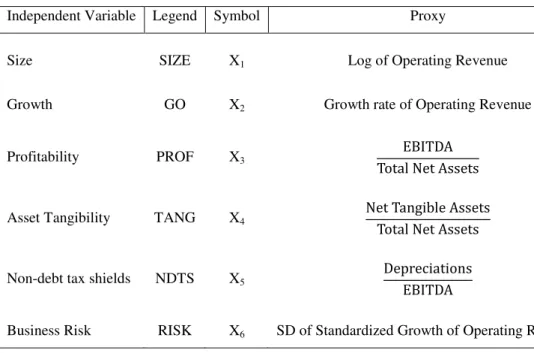
3.2.2. Independent Variables
This section focus on the definition of the independent variables to be used, considering
the different hypothesis made previously. For this investigation we choose the following
determinants of debt: size, given by the logarithm of operating revenue (Titman &
Wessels 1988, Barton et al 1989 and Ribeiro 2001 used turnover to measure the size;
however, due to data availability, we had to choose the operating revenue to rank size);
growth opportunities, given by the growth rate of operating revenue continuously
compounded; profitability given by the ratio between Earnings Before Interest, Taxes,
Depreciations and Amortizations (EBITDA) and net total assets; asset tangibility, given
by the ratio between net tangible assets and net total assets (Rajan & Zingales, 1995;
Rogão, 2006; Vieira & Novo, 2010; Silva, 2013); non-debt tax shields, given by the
ratio between depreciations and operating income; business risk, given by the standard
Table IV
Proxies of the independent variables
Independent Variable Legend Symbol Proxy
Size SIZE X1 Log of Operating Revenue
Growth GO X2 Growth rate of Operating Revenue
Profitability PROF X3
Asset Tangibility TANG X4
Non-debt tax shields NDTS X5
Business Risk RISK X6 SD of Standardized Growth of Operating Revenue
3.3. Methodology
To analyze the relationship between debt and its determinants, and consider the most
commonly approaches in the literature such as static panel models, namely, pooled OLS
regression and models admitting the existence of non-observable individual effects,
which can be random or fixed. These models differ mainly in the constant part of the
model specification and in the error term. In general, panel data models are a
combination of cross-section data with time series, gathering sectional observations of
different companies for multiple periods of time.
In the OLS method, the purpose is to estimate the beta parameters that minimize the
sum of squared residuals, this is the differences between the observed and estimated
values should be minimal. The estimated parameters represent linear functions of the
to be homoscedastic and non autocorrelated, which allows linear unbiased and
consistent estimators (Greene, 2008). If the heterogeneity in the data is ignored, the bias
will be great and opting for an OLS model may not be the best option.
In this case, it will be more appropriate to use alternative models, such as the fixed
effects model or the random effects model.
In the fixed effects model, the estimation is done assuming that the heterogeneity of
individuals (companies) is captured in the constant part, keeping the assumption of
homogeneity of observations (Greene, 2008). Fixed effects estimator is called either
‘Least Squares Dummies Variable (LSDV)’estimator or ‘Within Group’ estimator.
The random effects model considers the constant term not as a fixed parameter, but as
an unobservable random parameter. The model parameters are estimated by the method
of generalized least squares (Greene, 2008).
3.4.The Models
Considering the determinants of debt defined previously in this study and the three
proxies representative of the debt ratio, the evaluation of a pooled OLS regression can
be presented through the following models:
with:
i= 1, …, 87;
t = 1,…,5;
Where Y represents the dependent variables of the debt ratio, i represents each company
of the sample, t represents the period of time, represents an unobserved random
variable, the regression parameters to be estimated, is a industry dummy variable
(takes value 1 when the company belongs to the manufacturing sector and 0, otherwise),
represents a listed company dummy variable (assumes value 1 when the company is
listed on the Portuguese stock exchange and 0, otherwise), are temporal dummy
variables that measure the impact of possible macroeconomic alterations on company
debt, and at last is the error term not explained by the model, assumed to have a
normal distribution.
Considering the existence of non-observable individual effects, we have the following
models:
where, , with being companies’ non-observable individual effects.
The Breusch-Pagan test is used to test for heteroskedasticity in a linear regression
model. It tests whether the estimated variance of the residuals from a regression are
dependent on the values of the independent variables. Under the null hypothesis the
error variances are all equal (homoscedasticity), against the alternative that the error
variances are a multiplicative function of one or more variables.
To test if the best approach relies on a random effects or fixed effects model,
researchers often use a Hausman test, checking if there is a correlation between the
specific effect and the explanatory/independent variables. Under the null hypothesis
non-observable individual effects are uncorrelated with the explanatory variables,
whereas on the alternative hypothesis there is correlation between the non-observable
individual effects and the explanatory variables. Not rejecting the null hypothesis,
means the p-value is not significant (superior to 0.05) and that we should favor the
random effects model due to higher efficiency and consistency, while under the
alternative hypothesis, although a fixed effects model can be inefficient, is consistent
4.
Discussion of Empirical Results
Table a.2 (in appendix) reports the Pearson correlations among the variables used in this
study. The higher levels of correlation can be found between Size and Profitability
(0.180), Growth and Profitability (0.162), Growth and Tangibility (0.133), and Growth
and Non-Debt Tax Shields (0.108). Although these correlations are statistically
significant, the coefficients are all bellow 50% which does not imply multicollinearity
problems. The remaining values are quite low and close to zero which does not
compromise the analysis.
From the summary of descriptive statistics (table a.3 in appendix), we highlight the
average of the different indicators that represent the level of indebtness (46% to the total
debt, 13% for the long-term debt and 34% for short-term debt). The average short-term
debt is more than two times higher than the average of long-term debt. This indicator
reflects the poor dynamism of the Portuguese capital market during the period in
analysis, due to the great reliance that companies had on the banking system. The
graphic below, show us a clear declining of the debt ratio over time, specially
observable from 1986 and for the short-term period, which could mean that companies
no longer seek the banks as the only and major source of financing.
55.40% 56.01% 45.22%
36.79% 37.29% 14.61% 16.06%
13.02%
8.45% 10.51%
40.79% 39.95%
32.20%
28.34% 26.78%
1984 1985 1986 1987 1988
Tables a.4, a.5 and a.6 (in appendix) present the results from the estimated regression
models for each dependent variables considering the OLS, RE and FE (with and without
temporal dummies), as well as the results of F, Breusch-Pagan and Hausman tests. The
results show that the most suitable model for regressions Y1 and Y3 was the FE method,
once the null hypothesis of the F test is rejected, meaning that the pooled OLS model is
not the most appropriate one. Breusch-Pagan test confirms this result since the
existence of homoscedasticity is rejected. Finally, on the Hausman test we reject that
the differences in the coefficients are not systematic and opt for the fixed effects model.
For regression Y2, we reject the null hypothesis of the F and Breush-Pagan tests, which
states that the OLS model is not adequate. The difference is in the Hausman test, where
we do not reject the null, so the best model is the RE. In general, given the obtained
values, we notice no significant differences between the results of the different
regressions. Indeed, apart a few exceptions, the regressions are affected by the same
determinants and the constant term does not seem to have a meaningful importance in
explaining the majority of the dependent variables.
The coefficient of determination (R2) measures how close the data are to the fitted
regression model. The results of the fixed effects model for total debt (table a.7 in
appendix) presents a R2 of 0.785, which means that 78.5% of the total variability in total
debt is explained by the independent variables in the regression model. The determinant
factors of the total debt ratio are the following: size, profitability and asset tangibility.
As expected, size and asset tangibility had a positive relation with leverage of,
respectively, β1=7.7% and β4=39.4%. The results for profitability are also in line with
the established hypothesis, with a negative relation with the debt level of β3=23.6%.The
coefficient value is very close to zero (β5=0.4%) and the sign is not the expected in the
hypothesis previously established. Bradley et al. (1984) also expected a negative
correlation however the results presented a positive coefficient. For the other
independent variables there are no more statistically significant values, except the
variables business risk and quoted dummy when temporal dummies were not
considered.
Table a.8 (in appendix) presents the results for regression Y2,when the long-term debt
ratio is assumed as the dependent variable. As mentioned above, the most appropriated
model for this regression is the random effects panel model.The results reveal that the
variables size, growth, asset tangibility, non-debt tax shields and business risk have an
influence on the dependent variable.Regarding the expected signs of these relations, the
variables growth and non-debt tax shields did not correspond to the ones observed. It is
also noteworthy that only the variable asset tangibility has a significant relation with the
debt level, with a coefficient value of β4=21% and with a positive sign, as expected. The
remaining independent variables present no statistically significant value.
Finally, table a.9 (in appendix) provides us the results of the regression Y3, using the
short-term debt ratio as the dependent variable. Considering the fixed effects model, the
value of this coefficient indicates that 79.4% of the total variability in short-term debt is
explained by the independent variables in the regression model. The determinants
factors of the short-term debt ratio are the following: size, growth, profitability, asset
tangibility and business risk. As expected, size, growth and asset tangibility had a
positive relation with leverage of, respectively, β1=5%, β2=3.4% and β4=20.1%. The
determinant factor, although the sign is not the expected and with a coefficient of
β6=3.1%. The other independent variables present no statistically significant values,
except the variable quoted dummy when we do not consider temporal dummies in the
model.
Table X summarizes the results obtained.
Table X
Expected and Observed Relations in the Regression Models
Y1 Y2 Y3
Hypothesis Expected Relations Observed Significant1 Relations Expected Relations Observed Significant1 Relations Expected Relations Observed Significant1 Relations Debt and the size of a
firm. + + + + + +
Debt and the growth of
a firm. + + - + +
Debt and the
profitability. - - - -
Debt and the level of
tangible assets. + + + + + +
Debt and the non-debt
tax shields. - + - + -
Debt and the business
risk. - - - -
1 for values equal or inferior to 5%
After analyzing the empirical results, we looked at the same results in the light of the
theories of capital structure addressed in Chapter 2, in particular, the pecking order
5.
Conclusions
This dissertation investigates the capital structure determinants of 87 Portuguese listed
firms covering the period between 1984 and 1988. The aim was to contribute to a
deeper understanding of the Portuguese case during a period barely studied.
Considering the variables suggested by the main theories of capital structure, six
potential determinants were analyzed: size, growth opportunities, profitability, asset
tangibility, non-debt tax shields and business risk. We found that the pooled OLS
regression was not the most appropriate method and consequently, panel models of
random or fixed effects were considered. In general, the results obtained by the different
regressions are similar concerning the signs and level of significance of the parameters.
The models presented a good explanatory power with high values for the coefficient of
determination. Results show that size and asset tangibility are significant determinants
of the capital structure for the sample in analysis. Size and debt presented a positive and
statistically significant relationship allowing us to conclude that larger firms turn more
to debt than smaller firms, since they are able to access better credit conditions and are
less likely to go bankrupt. Growth shows a negative relationship long-term and
short-term debt measures, meaning that companies with the highest growth rate of its assets
also tend to be less indebted. However, for total debt this variable has no significance.
Profitability by assuming a negative significant relationship with total debt confirms the
pecking-order theory, suggesting that the most profitable Portuguese listed companies
resort less to debt, preferring on first place internal financing. For asset tangibility
variable, we found that companies with greater proportion of tangible assets in its total
support to the current literature for the business risk variable, which states an inverse
relationship with debt.
To summarize, we reach the conclusion that the debt level of Portuguese listed
companies does not vary randomly, reflecting a behavior described by the theories of
Trade-off and Pecking Order.
In future research, it would be interesting to fill the lack of information about
Portuguese firms on the period of analysis, as well as it would be interesting to make a
connection between that information and the nineties decade studies. Additionally,
References
Antão, P. & Bonfim, D. (2008). Capital Structure Decisions in the Portuguese Corporate Sector. Banco de Portugal Financial Stability Report 2008.
Baker, M. & Wurgler, J. (2002). Market timing and capital structure. The Journal of Finance 57, 1-32.
Bancel, F. & Mittoo, U. (2004). Cross-country determinants of capital structure choice: a survey of European firms. Financial Management 33(4), 103-132.
Barton, S. L., Hill, N. C. & Sundaram, S. (1989). An Empirical Test of Stakeholder Theory Predictions of Capital Structure. Financial Management 18(1), 36-44.
Berk, J. & DeMarzo, P. (2013). Corporate Finance, 3rd Ed. S.I.: Pearson.
Booth, L., Aivazian, V., Demirguc-Kunt, A. & Maksimovic, V. (2001). Capital structures in developing countries. The Journal of Finance 56(1), 87-130.
Bradley, M., Jarrell, G. & Kim, E. H. (1984). On the existence of an optimal capital structure: Theory and evidence. The Journal of Finance 39, 857–878.
Brennan, M. J. & Eduardo, S. (1978). Finite difference methods and jump processes arising in the pricing of contingent claims: A synthesis. Journal of Financial and Quantitative Analysis 20, 461–473.
Chung, K. H. (1993). “Asset characteristics and corporate debt policy: an empirical
test”. Journal of Business Finance & Accounting 20 (1), 83-98.
Couto, G. & Ferreira, S. (2010). Os determinantes da estrutura de capital de empresas do PSI 20. Revista Portuguesa e Brasileira de Gestão 9(1-2), 26-38.
DeAngelo, H. & Masulis, R. W. (1980). Optimal capital structure under corporate and personal taxation. Journal of Financial Economics 8, 3-29.
Donaldson, G. (1962). Corporate debt capacity: a study of corporate debt policy and the determination of corporate debt capacity. The American Economic Review 52, 628-9.
Durand, D. (1952). Costs of Debt and Equity Funds for Business: Trends and Problems of Measurement” in Nat. Bur. Econ. Research. Conference on Research in Business Finance, 215-47.
Frank, M. & Goyal, V. (2004). The effect of market conditions on capital structure adjustment. Finance Research Letters 1, 47-55.
Gaud, P., Jani, E., Hoesli, M. & Bender, A. (2005). The capital structure of Swiss companies: an empirical analysis using dynamic panel data. European Financial Management 11, 51-69.
Gomes, A., Botelho, F., Silva J. C. & Vasconcelos, J. (1987). Guia da Bolsa, Lisbon: Fragmentos.
Graham, J. & Harvey, C. (2001). The theory and practice of corporate finance: evidence from the field. Journal of Financial Economics 60, 187-243.
Greene, W. H. (2008). Econometric Analysis, 6th Ed. Prentice Hall.
Harris, M. & Raviv, A. (1991). The Theory of Capital Structure. The Journal of Finance 46(1), 297-355.
Haugen, R. A. & Senbet, L. W. (1988). Bankruptcy and Agency Costs: Their Significance to Theory of Optimal Capital Structure. Journal of Financial and Quantitative Analysis 23(1), 27-39.
Jensen, Michael C. (1986). Agency Costs of Free Cash Flow, Corporate Finance, and Takeovers. The American Economic Review 76(2), 323-329.
Jorge, S. & Armada, M. (2001). Factores determinantes do endividamento: uma análise em painel. Revista de AdministraçãoContemporânea 5(2), 9-31.
Kim, E. Han (1978). A Mean-Variance Theory of Optimal Capital Structure and Corporate Debt Capacity. The Journal of Finance 33(1), 45-63.
Kim, W. S. & Sorensen, E. H. (1986). Evidence on the impact of the agency costs of debt on corporate debt policy. Journal of Financial and Quantitative Analysis 21 (2),
131-144.
Kraus A. & Litzenberger R. (1973). A state preference model of optimal financial leverage. The Journal of Finance 28, 991-921.
Kremp, E., Stöss, E., Gerdesmeier, D. (1999). Estimation of a debt function: evidence from French and German firm panel data. In Sauvé, A., Scheuer, M. (ed.) Corporate
finance in Germany and France. A joint research project of Deutsche Bundesbank and the Banque de France, SSRN working paper.
Mackie-Mason, J. K. (1990). Do Taxes Affect Corporate Financing Decisions?. The Journal of Finance 45(5), 1471-1493.
Modigliani, F. & Miller, M. (1958). The Cost of Capital, Corporation Finance and the Theory of Investment. American Economic Review, 97-261.
Modigliani, F. & Miller, M. (1963). Corporate Income Taxes and the Cost of Capital: a Correction. American Economic Review, 433-443.
Myers, S. C. (1984). The capital structure puzzle. The Journal of Finance 39, 575-92.
Myers, S. C. (1977). Determinants of corporate borrowing. Journal of Financial Economics 5, 147-175.
Myers, S. & Majluf, N. (1984). Corporate financing and investments decisions when firms have information that investors do not have. Journal of Financial Economics
39(3), 187-222.
Myers, S. C. (2001). Capital structure. Journal of Economic Perspectives 15 (2),
81-102.
Rajan, R. & Zingales, L. (1995). What Do We Know about Capital Structure? Some Evidence from International Data. The Journal of Finance 50(5), 1421-1460.
Rita, R. M. S. (2003). As teorias de estruturas de capitais: A evidência empírica das empresas Portuguesas. Évora: Dissertação do Mestrado em Gestão de Empresas, Universidade de Évora.
Scott, J. (1977). A theory of optimal capital structure. Bell Journal of Economics 32,
33-54.
Serrasqueiro, Z. & Rogão, M. (2009). Capital structure of listed Portuguese companies: determinants of debt adjustment. Review of Accounting and Finance 8(1), 54-75.
Silva, S. (2013). Determinantes da Estrutura de Capitais: evidência empírica das empresas portuguesas cotadas na Euronext Lisbon. Porto: Dissertação de Mestrado, Faculdade de Economia da Universidade do Porto.
Titman, S. & Wessels, R. (1988). The determinants of capital structure choice. The Journal of Finance 43(1), 1-19.
Vieira, E. S. & Novo, A. (2010). A estrutura de capital das PME: evidência no mercado português. Estudos do ISCA, 4(2).
Vieira, E. S. (2013). Capital Structure Determinants in the Context of Family Firms.
Proceedings in ARSA-Advanced Research in Scientific Areas 1, 219-228.
Warner, J. (1977). Bankruptcy Costs: Some Evidence. The Journal of Finance 32(2),
Appendix
Table a.1
List of Companies
List of Companies Industry
1 ALCO - Algodoeira Comercial e Industrial, S.A. 3
2 ARBORFIL - Fiação de Trofa 3
3 CABELTE - Cabos Eléctricos e Telefónicos 3
4 CEL-CAT - Fábrica Nacional de Condutores Eléctricos, SARL 3
5 Cinca - Companhia Industrial de Ceramica, S.A. 3
6 CIPAN - C.ª Ind. Prod. Antibióticos 3
7 Companhia Aveirense de Moagens 3
8 Companhia de Celulose do Caima, S.A. 3
9 Companhia Industrial de Resinas Sintéticas Cires, S.A. 3 10 Companhia Nacional de Fiação e Tecidos de Torres Novas 3
11 Companhia Portuguesa de Amidos – COPAM 3
12 Companhia Portuguesa do Cobre, S.A. 3
13 Companhia Portuguesa Higiene 3
14 Companhia Portuguesa Rádio Marconi 7
15 Construções Metalomecânicas Mague 3
16 COTAPO - Empreendimentos Comerciais e Industriais 8
17 CPPC - Companhia do Papel de Porto de Cavaleiros 3
18 Crisal - Cristais de Alcobaça, S.A. 3
19 EFACEC, Empresa Fabril de Máquinas Electricas, S.A. 3
20 EMPOR - Empreendimentos Comerciais e Financeiros 6
21 ENGIL - Soc. Construção Civil 5
22 Estoril-Sol 9
23 F. Ramada, Aços e Industrias, S.A. 3
24 Fábricas Triunfo, S.A. 3
25 FEPSA - Feltros Portugueses 3
26 Fiação de Algodões de Coimbra – FIACO 3
27 FINAGRA - Sociedade Industrial e Agrícola 1
28 Fisipe - Fibras Sintéticas de Portugal, S.A. 3
29 FITOR - Comp. Port. De Têxteis 3
30 Fosforeira Portuguesa 3
31 G.A.P. - Gestão Agro-Pecuária 1
32 INAPA [INAPA - Indústria Nacional de Papéis, SARL] 3
33 INDASA - Indústria de Abrasivos 3
35 INÔ – Supermercados 6
36 JÚPITER - Indústria Hoteleira 6
37 Lisnave - Estaleiros Navais de Lisboa, S.A. 3
38 LITHO FORMAS PORTUGUESA - Impres. Cont. e Múlt. 3
39 LUSOTUR - Sociedade Financeira de Turismo 8
40 LUZOSTELA - Indústria de Abrasivos e Colas 3
41 MABOR - Manufactura Nacional de Borracha, S.A. 3
42 MUNDICENTER - Soc. Imobiliária 8
43 NOVOPAN - Empresa Produtora de Aglomerados de Madeiras 3 44 Oliveira & Ferreirinhas - Indústrias Metalurgicas, S.A. 3
45 ORBITUR - Intercâmbio de Turismo 6
46 Papelaria Fernandes - Indústria e Comércio 6
47 Petróleo Mecânica Alfa 3
48 Pirites Alentejanas 2
49 POLIMAIA - Sociedade Industrial Química 3
50 Proalimentar - Companhia de Produtos Alimentares do Centro 3 51 Produtos Alimentares António & Henrique Serrano 3
52 PROEMBA - Produtos de Embalagem 3
53 REDITUS - Processamento Aut. De Informação 3
54 S.P.C. - Serv. Português de Contentores 7
55 SABEL - Santos & Bento 6
56 SALVADOR CAETANO - Ind. Met. Veículos Transportes 3
57 SICEL - Soc. Industrial de Cereais 3
58 Sociedade Comercial Orey Antunes 7
59 Sociedade da Água do Luso 3
60 Sociedade das Águas da Curia 9
61 Sociedade de Construções Amadeu Gaudêncio 5
62 Sociedade de Construções Soares da Costa 5
63 Sociedade de Empreitadas Somague 5
64 Sociedade de Iniciativa e Aproveitamentos Florestais - SIAF 3 65 Sociedade de Representações Santos, Guimarães & Oliveira 6
66 Sociedade Figueira-Praia 9
67 Sociedade Industrial de Vila Franca, S.A. 3
68 Sociedade Portuguesa de Computadores em Tempo Dividido (Time Sharing) 8
69 Sociedade Turística da Penina 6
70 Soja de Portugal, S.A. 3
71 SOLIDAL - Condutores Eléctricos 3
72 SOLVERDE - Soc. Inv. Tur. Costa Verde 9
75 SONAGI - Soc. Nac. De Gestão e Investimento 8 76 SOPETE - Sociedade Poveira de Empreendimentos Turísticos 9
77 Soporcel - Sociedade Portuguesa de Celulose, S.A. 3
78 Sotave - Sociedade Têxtil dos Amieiros Verdes 3
79 SUMOLIS - Comp. Ind. Frutas e Bebidas 3
80 Supermercados A. C. Santos 6
81 TELECINE-MORO - Soc. Produtora de Filmes 9
82 TERNOR - Soc. Exploração Terminais 7
83 Têxteis Moura & Matos 3
84 TRANSBEL - Transportes e Trânsitos Internacionais 7
85 TRANSINSULAR - Transp. Marítimos Insulares 7
86 Transmotor 6
87 Vidago, Melgaço e Pedras Salgadas 3
Legend:
1 Agriculture, Forestry, Fishing and Hunting 2 Mining and Quarrying
3 Manufacturing 4 Public Utilities 5 Construction
Table a.2 Correlation Matrix Debt/ Asset Long-term Debt/Asset Current Debt/ Asset
Size Growth Profitability TangibilityAsset Tax ShieldsNon-Debt Business Risk
Pearson
Correlation 1 .445** .765** .220** .121* .118* .094 .052 -.143**
Sig.
(2-tailed) .000 .000 .000 .011 .013 .050 .283 .003
Pearson
Correlation .445** 1 -.236** .020 .050 -.005 .324** .138** -.062
Sig.
(2-tailed) .000 .000 .682 .298 .919 .000 .004 .200
Pearson
Correlation .765** -.236** 1 .225** .095* .132** -.131** -.043 -.110*
Sig.
(2-tailed) .000 .000 .000 .047 .006 .006 .372 .021
Pearson
Correlation .220** .020 .225** 1 .039 .180** -.142** -.113* -.133**
Sig.
(2-tailed) .000 .682 .000 .413 .000 .003 .018 .005
Pearson
Correlation .121* .050 .095* .039 1 .108* .133** .162** -.201**
Sig.
(2-tailed) .011 .298 .047 .413 .024 .005 .001 .000
Pearson
Correlation .118* -.005 .132** .180** .108* 1 .070 -.037 -.156**
Sig.
(2-tailed) .013 .919 .006 .000 .024 .143 .438 .001
Pearson
Correlation .094 .324** -.131** -.142** .133** .070 1 .010 -.038
Sig.
(2-tailed) .050 .000 .006 .003 .005 .143 .842 .424
Pearson
Correlation .052 .138** -.043 -.113* .162** -.037 .010 1 -.085
Sig.
(2-tailed) .283 .004 .372 .018 .001 .438 .842 .076
Pearson
Correlation -.143** -.062 -.110* -.133** -.201** -.156** -.038 -.085 1
Sig.
(2-tailed) .003 .200 .021 .005 .000 .001 .424 .076
*. Correlation is significant at the 0.05 level (2-tailed).
Debt/ Asset Long-term Debt/Asset Current Debt/ Asset Size Growth Profitability Asset Tangibility Non-Debt Tax Shields Business Risk
Table a.3
Summary of Descriptive Statistics
Variables Min. Max. Mean Std. Deviation
Y1 .0023 1.0237 .4614 .2146
Y2 .0000 .7248 .1253 .1422
Y3 .0013 .9222 .3361 .1978
SIZE .0000 8.3595 6.8589 .7390
GO -2.6640 3.4363 .1977 .3641
PROF -.0843 .6648 .1597 .1011
TANG .0017 1.4659 .3408 .2154
NDTS -37.7384 68.1016 .3907 3.7896
Table a.4
Results of Y1 regression model
Dependet Variable: Y1 = Debt to Asset
I II I II I II
Constant 0.026 -0.061 0.046 -0.097 0.150 -0.059
(-0.278) (-0.667) (0.442) (-0.994) (1.240) (-0.522)
Size 0.075 *** 0.086 *** 0.059 *** 0.085 *** 0.042 ** 0.077 ***
(5.434) (6.442) (3.835) (5.749) (2.257) (4.426)
Growth 0.040 0.037 0.010 -0.003 0.005 -0.010
(1.498) (1.417) (0.515) (-0.174) (0.268) (-0.569)
Profitability −0.062 -0.051 -0.097 -0.146 -0.169 -0.236 **
(−0.603) (-0.516) (-0.946) (-1.532) (-1.461) (-2.237)
Asset Tangibility 0.085 * 0.086 ** 0.232 *** 0.250 *** 0.393 *** 0.394 ***
(1.916) (2.004) (4.174) (4.769) (5.419) (5.896)
Non-debt tax shields 0.003 0.003 0.003 * 0.003 * 0.004 ** 0.004 **
(1.029) (-1053) (1.748) (1.888) (2.136) (2.304)
Business Risk -0.029 -0.006 -0.39 * -0.012 -0.040 * -0.014
(-1095) (-0.223) (-1.906) (-0.609) (-1.893) (-0.737)
Industry dummy 0.042 ** 0.036 * 0.053 0.044 --
--(1.994) (-1.758) (1.493) (1.262)
Quoted dummy -0.141 *** -0.046 -0.158 *** -0.038 * -0.151 *** -0.031
(-7.276) (-1.871) (-10.49) (-1.860) (-9.672) (-1.482)
Temporal dummies No Yes No Yes No Yes
R2 0.193 0.266 0.732 0.785
R2 (adj.) 0.178 0.245
F-stat. (1) 12.77 *** 12.75 ***
Breusch-Pagan 262.21 *** 318.78 ***
Hausman 26.488 *** 22.402 **
OLS Random Effects Fixed Effects
Table a.5
Results of Y2 regression model
*** p-value significant at 1%; ** p-value significant at 5% and * p-value significant at 10% (with statistics t-values in brakets)
Dependet Variable: Y2 = Long-Term Debt to Asset
I II I II I II
Constant -0.056 -0.065 -0.044 -0.065 -0.059 -0.087
(-0.876) (-1.014) (-0.625) (-0.913) (-0.704) (-1.016)
Size 0.021 ** 0.022 ** 0.021 ** 0.023 ** 0.025 * 0.028 **
(2.306) (2.347) (2.039) (2.145) (1.956) (2.067)
Growth -0.009 -0.011 -0.035 *** -0.038 *** 0.041 *** -0.044 ***
(-0.521) (-0,602) (-2.637) (-2.882) (-3.056) (-3.319)
Profitability -0.118 * -0.113 -0.083 -0.085 -0.053 -0.064
(-1.705) (-1.639) (-0.175) (-1.210) (-0.651) (-0.787)
Asset Tangibility 0.216 *** 0.218 *** 0.201 *** 0.210 *** 0.177 *** 0.193 ***
(7.197) (7.249) (5.319) (5.534) (3.491) (3.778)
Non-debt tax shields 0.005 *** 0.005 *** 0.004 *** 0.004 *** 0.004 *** 0.004 ***
(2.990) (3.083) (3.136) (3.307) (2.748) (2.938)
Business Risk -0.007 -0.007 -0.038 *** -0.038 *** -0.047 *** -0.045 ***
(-0.404) (-0.372) (-2.721) (-2.631) (-3.197) (-3.064)
Industry dummy 0.012 0.011 0.006 0.005 --
--(0.837) (0.774) (0.251) (0.211)
Quoted dummy -0.051 *** -0.035 ** -0.050 *** -0.025 * 0.051 *** -0.024
(-3.875) (-2.001) (-4.837) (-1.684) (-4.722) (-1.466)
Temporal dummies No Yes No Yes No Yes
R2 0.163 0.173 0.703
R2 (adj.) 0.148 0.150
F-stat. (1) 10.40 *** 7.379 ***
Breusch-Pagan 253.31 *** 263.62 ***
Hausman 13.18 * 13,50
Independent variables
Table a.6
Results of Y3 regression model
Dependet Variable: Y3 = Current Debt to Asset
I II I II I II
Constant 0.030 0.004 0.102 -0.028 0.210 * 0.029
(0.329) (0.088) (1.073) (-0.305) (1.967) (0.282)
Size 0.053 *** 0.064 *** 0.034 ** 0.060 *** 0.016 0.050 ***
(4.068) (4.972) (2.431) (4.363) (1.014) (3.154)
Growth 0.050 * 0.048 * 0.045 *** 0.035 ** 0.046 *** 0.034 **
(1.939) (1.910) (2.652) (2.267) (2.725) (2.183)
Profitability 0.056 0.063 -0.031 -0.080 -0.116 -0.173 *
(0,575) (0.660) (-0.328) (-0.909) (-1.143) (-1.812)
Asset Tangibility -0.131 *** -0.132 *** 0.060 0.064 0.217 *** 0.201 ***
(-3.084) (-3.210) (1.158) (1.302) (3.391) (3.333)
Non-debt tax shields -0.002 -0.003 -0.001 -0.001 0.000 0.000
(-1.036) (1.157) (-0.330) (-0.523) (0.250) (0.063)
Business Risk -0.022 0.001 -0.001 0.028 0.007 0.031 *
(-0.863) (0.040) (0.056) (1.643) (0.382) (1.780)
Industry dummy 0.030 0.025 0.050 0.042 --
--(1.500) (1.259) (1.397) (1.183)
Quoted dummy -0.090 *** -0.011 -0.107 *** -0.012 -0.099 *** -0.008
(-4.890) (-0.481) (-8.005) (-0.651) (-7.246) (-0.400)
Temporal dummies No Yes No Yes No Yes
R2 0.137 0.197 0.755 0.794
R2 (adj.) 0.120 0.175
F-stat. (1) 8.431 *** 8.654 ***
Breusch-Pagan 313.41 *** 361.16 ***
Hausman 25.33 *** 19.88 **
Independent variables