WO R K I N G PA P E R S E R I E S

WO R K I N G PA P E R S E R I E S

N O. 4 9 4 / J U N E 2 0 0 5

CROSS-COUNTRY

EFFICIENCY OF

SECONDARY EDUCATION

PROVISION

A SEMI-PARAMETRIC

ANALYSIS WITH

NONDISCRETIONARY

INPUTS

In 2005 all ECB publications will feature a motif taken from the

€_{50 banknote.}

W O R K I N G PA P E R S E R I E S

N O. 4 9 4 / J U N E 2 0 0 5

This paper can be downloaded without charge from http://www.ecb.int or from the Social Science Research Network electronic library at http://ssrn.com/abstract_id=726688.

CROSS-COUNTRY

EFFICIENCY OF

SECONDARY EDUCATION

PROVISION

A SEMI-PARAMETRIC

ANALYSIS WITH

NONDISCRETIONARY

INPUTS

by António Afonso

and Miguel St. Aubyn

-© European Central Bank, 2005 Address

Kaiserstrasse 29

60311 Frankfurt am Main, Germany

Postal address

Postfach 16 03 19

60066 Frankfurt am Main, Germany

Telephone

+49 69 1344 0

Internet

http://www.ecb.int

Fax

+49 69 1344 6000

Telex

411 144 ecb d

All rights reserved.

Reproduction for educational and non-commercial purposes is permitted provided that the source is acknowledged.

The views expressed in this paper do not necessarily reflect those of the European Central Bank.

The statement of purpose for the ECB Working Paper Series is available from the ECB website, http://www.ecb.int.

C O N T E N T S

Abstract 4

Non-technical summary 5

1 Introduction 7

2 Motivation and literature on education

efficiency 8

3 Analytical methodology 12

3.1 DEA framework 12

3.2 Non-discretionary inputs and the

DEA/Tobit two-steps procedure 13

3.3 Non-discretionary inputs and bootstrap 15

4 Empirical analysis 18

4.1 Data and indicators 18

4.2 DEA efficiency results 19

4.3 Explaining inefficiency – the role of

non-discretionary inputs 21

5 Conclusion 28

Appendix – Additional Tobit and bootstrap results 30

References 32

Annex – Data and sources 34

Abstract

We address the efficiency of expenditure in education provision by comparing the output (PISA results) from the educational system of 25, mostly OECD, countries with resources employed (teachers per student, time spent at school). We estimate a semi-parametric model of the education production process using a two-stage procedure. By regressing data envelopment analysis output scores on non-discretionary variables, both using Tobit and a single and double bootstrap procedure, we show that inefficiency is strongly related to GDP per head and adult educational attainment.

Non-technical summary

Education is one of the most important services provided by governments in almost every country. According to OECD data, OECD countries expended an average of 6.2 percent of GDP in 2001 on education institutions, of which 4.8 percent of GDP were from public sources. Additionally, education spending is predominantly public in OECD countries, and for all education levels. Data for 30, mostly OECD, countries in 2001, shows that public resources accounted on average for some 88% of the total financing of education provision.

In a general sense, education provision is efficient if its producers make the best possible use of available inputs, and the sole fact that educational inputs weight heavily on the public purse would call for a careful efficiency analysis. An education system not being efficient would mean either that results (or “outputs”) could be increased without spending more, or else that expense could actually be reduced without affecting the outputs, provided that more efficiency is assured. Research results presented here indicate that there are cases where considerable improvements can be made in this respect.

In this paper we systematically compare the output from the secondary educational system of 25 countries with resources employed (number of teachers per student, time spent at school). Education achievement, the output, is measured by the performance of 15-year-olds on the OECD PISA reading, mathematics, problem solving, and science literacy scales in 2003. Using data envelopment analysis (DEA), we derive a theoretical production frontier for education. In the most favourable case, a country is operating on the frontier, and is considered as efficient. However, most countries are found to perform below the frontier and an estimate of the distance each country is from that borderline is provided – the so-called efficiency score.

Results from the first-stage imply that inefficiencies may be quite high. On average and as a conservative estimate, countries could have increased their results by 11.6 percent using the same resources, with a country like Indonesia displaying a waste of 44.7 percent.

Our second stage procedures show that GDP per head and parents’ educational attainment are highly and significantly correlated to output scores – a wealthier and more cultivated environment are important conditions for a better student performance. Moreover, it becomes possible to correct output scores by considering the harshness of the environment where the education system operates. Country rankings and output scores derived from this correction are substantially different from standard DEA results.

1. Introduction

In this paper we systematically compare the output from the educational system of 25 countries with resources employed (number of teachers per student, time spent at school). Using data envelopment analysis (DEA), we derive a theoretical production frontier for education. In the most favourable case, a country is operating on the frontier, and is considered as efficient. However, most countries are found to perform below the frontier and an estimate of the distance each country is from that border line is provided – the so-called efficiency score. Moreover, estimating a semi-parametric model of the education production process using a two-stage approach, we show that inefficiency in the education sector is strongly related to two variables that are, at least in the short- to medium run, beyond the control of governments. These are the family economic background and the education of parents.

In methodological terms, a two-stage approach has become increasingly popular when DEA is used to assess efficiency of decision-making units (DMUs). In some cases, this approach has been applied to the education sector4, but rarely in an international framework with whole countries as units of observation. The most usual two-stage approach has been recently criticised in statistical terms.5 The fact that DEA output scores are likely to be biased, and that the environmental variables are correlated to output and input variables, recommend the use of bootstrapping techniques, which are well suited for the type of modelling we apply here. Therefore, we employ both a more usual DEA/Tobit approach and single and double bootstrap procedures suggested by Simar and Wilson (2004). Our paper is one of the first application examples of this very recent technique. Our results following this technique are compared to the ones arising from the more traditional one.

The paper is organised as follows. In section two we provide motivation and briefly review some of the literature and previous results on education provision efficiency. Section three outlines the methodological approach used in the paper and in section four we present and discuss the results of our efficiency analysis. Section five provides conclusions.

4

See Ruggiero (2004) for a survey.

5

2. Motivation and literature on education efficiency

Education is one of the most important services provided by governments in almost every country. According to OECD (2004a), OECD countries expended an average of 6.2 percent of GDP in 2001 on education institutions, of which 4.8 percent of GDP were from public sources. In a general sense, education provision is efficient if its producers make the best possible use of available inputs, and the sole fact that educational inputs weight heavily on the public purse would call for a careful efficiency analysis. An education system not being efficient would mean either that results (or “outputs”) could be increased without spending more, or else that expense could actually be reduced without affecting the outputs, provided that more efficiency is assured. Research results presented here indicate that there are cases where considerable improvements can be made in this respect.

Table 1 – Public expenditure on education, 2001 (% of total expenditure in each level)

Pre-primary education Primary and secondary education Tertiary education

All levels of education

Australia 68.9 84.4 51.3 75.6

Austria 79.3 96.3 94.6 94.4

Belgium 96.6 95.0 84.1 93.0

Czech Republic 91.8 92.1 85.3 90.6

Denmark 81.7 98.0 97.8 96.1

Finland 91.0 99.1 96.5 97.8

France 95.9 93.0 85.6 92.0

Germany 62.3 81.1 91.3 81.4

Greece na 91.4 99.6 94.2

Hungary 90.6 93.1 77.6 89.0

Iceland na 95.3 95.0 91.7

Indonesia 5.3 76.3 43.8 64.2

Ireland 33.2 95.3 84.7 92.2

Italy 97.0 98.0 77.8 90.7

Japan 50.4 91.5 43.1 75.0

Korea 48.7 76.2 15.9 57.1

Mexico 86.7 87.2 70.4 84.6

Netherlands 98.2 95.1 78.2 90.9

Norway na na 96.9 95.9

Portugal na 99.9 92.3 98.5

Slovak Republic 97.4 98.5 93.3 97.1

Spain 83.4 93.3 75.5 87.8

Sweden 100.0 99.9 87.7 96.8

Switzerland na 84.8 na na

Thailand 97.8 na 82.5 95.6

Tunisia na 100.0 100.0 100.0

Turkey na na 95.8 na

United Kingdom 95.7 87.2 71.0 84.7

United States 68.1 93.0 34.0 69.2

Uruguay 81.3 93.5 99.5 93.4

Mean 78.3 92.2 79.3 88.2

Median 86.7 93.3 85.3 91.9

Minimum 5.3 76.2 15.9 57.1

Maximum 100.0 100.0 100.0 100.0

Standard deviation 24.3 6.8 21.8 10.8

Observations 23 27 29 28

Sources: Education at a Glance 2004, OECD – Tables B3.2a, B3.2b.

Notes: Public expenditure on education includes public subsidies to households attributable for educational institutions and direct expenditure on educational institutions from international sources. Private expenditure on education is net of public subsidies attributable for educational institutions. na – not available.

Concern with education also comes from the belief that this is an important source of human capital formation and therefore of economic growth, as suggested by economic theory.6 However, empirical work on this relationship has not been conclusive, and

6

the correlation between education and growth is not statistically significant in some published results.7 Most empirical work on this field has progressed by means of cross-country regressions where human capital quantity measured as the average number of years of schooling is one of the independent variables deemed to explain growth. Some researchers have found that quality matters for growth. Namely, Hanushek and Kimko (2000) and Barro (2001) showed that education quality, as measured by international comparative tests of skills, has a strong relationship with economic growth.

Moreover, the relevance of assessing the quality of public spending and redirecting it to more growth enhancing items is stressed in EC (2004) as being an important goal for governments to pursue. Additionally, there is also internationally a shift in the focus of the analysis from the amount of public resources used by a government, to the services delivered, and also to the outcomes achieved and their quality (see namely OECD (2003b)).

In our research, we measure and compare education output across countries using precisely the abovementioned type of quality measures – we resort to the most recent cross-nationally comparable evidence on student performance, the 2003 results from the Programme for International Student Assessment (PISA), launched by the OECD.8

Previous research on the international comparative performance of the public sector in general and of education systems in particular, including Afonso, Schuknecht and Tanzi (2003) for public expenditure in the OECD, St. Aubyn (2003) for education spending in the OECD and Gupta and Verhoeven (2001) for education and health in Africa, has already suggested that important inefficiencies are at work. All these studies use free disposable hull analysis (FDH) with inputs measured in monetary terms. Using both FDH and DEA analysis, Afonso and St. Aubyn (2005) studied efficiency in providing health and education in OECD countries using physically measured inputs and concluded that average input inefficiency varies between 0.859

7

See Benhabib and Spiegel (1994) and Pritchett (2001).

8

and 0.886 – if all countries were efficient, input usage could be reduced by about 13 percent without affecting output.

In a related but separate research strand, some authors have studied the determinants of schooling quality across countries using cross-country regressions, by specifying and estimating linear models for the relationship between schooling quality and its determinants. The former is measured by cross-country comparative studies assessing learning achievement. The latter include resources allocated to education (e. g. teachers per pupil or expenditures per student) and other factors that may affect the educational output, such as parents’ income or instruction level. Barro and Lee (2001) find that student performance is positively correlated to the level of school resources, such as pupil-teacher ratios, and also to family background (income and education of parents). Hanushek and Kimko (2000) and Hanushek and Luque (2003) find little or no evidence of a positive link from more resources allocated to the education system and test performance. However, they find that adult schooling levels have a positive and significant effect on student performance.

In this paper, we put these two strands of the literature together by estimating a semi-parametric model of the education production process using a two-stage approach. In a first stage, we determine the output efficiency score for each country, using the mathematical programming approach known as DEA, relating education inputs to outputs. In a second stage, these scores are explained using regression analysis. Here, we show that family background variables identified by previous authors are indeed highly correlated to inefficiency, i.e., they are significant “environmental variables”, using DEA jargon.9 They are, however, of a fundamentally different nature from input variables, in so far as their values cannot be changed in a meaningful spell of time by the DMU, here a country.

3. Analytical methodology

3.1. DEA framework

DEA, originating from Farrell (1957) seminal work and popularised by Charnes, Cooper and Rhodes (1978), assumes the existence of a convex production frontier. This frontier in the DEA approach is constructed using linear programming methods, the term “envelopment” stemming from the fact that the production frontier envelops the set of observations.10

DEA allows the calculation of technical efficiency measures that can be either input or output oriented. The purpose of an output-oriented study is to evaluate by how much output quantities can be proportionally increased without changing the input quantities used. This is the perspective taken in this paper. Note, however, that one could also try to assess by how much input quantities can be reduced without varying the output. The two measures provide the same results under constant returns to scale but give different values under variable returns to scale. Nevertheless, both output and input-oriented models will identify the same set of efficient/inefficient producers or DMUs.

The analytical description of the linear programming problem to be solved, output oriented and assuming variable returns to scale hypothesis, is sketched below. Suppose there are p inputs and q outputs for n DMUs. For the i-th DMU, yi is the

column vector of the outputs and xi is the column vector of the inputs. We can also

define X as the (p×n) input matrix and Y as the (q×n) output matrix. The DEA model is then specified with the following mathematical programming problem, for a given i-th DMU:

10

0 1 ' 1 to s. , ≥ = ≥ ≤ λ λ λ λ δ δ δ λ n X x Y y Max i i i i i

. (1)

In problem (1), δi is a scalar satisfyingδi ≥1. It is the efficiency score that measures

technical efficiency of the i-th unit as the distance to the efficiency frontier, the latter being defined as a linear combination of best practice observations. Withδi >1, the

decision unit is inside the frontier (i.e. it is inefficient), while δi =1 implies that the

decision unit is on the frontier (i.e. it is efficient).

The vector λ is a (n×1) vector of constants, which measures the weights used to compute the location of an inefficient DMU if it were to become efficient. The inefficient DMU would be projected on the production frontier as a linear combination of its peers using those weights. The peers are other DMUs that are more efficient and therefore used as references.

1

n is a n-dimensional vector of ones. The restriction n1'λ =1 imposes convexity of

the frontier, accounting for variable returns to scale. Dropping this restriction would amount to admit that returns to scale were constant.

Notice that problem (1) has to be solved for each of the n DMUs in order to obtain n

efficiency scores.

3.2. Non-discretionary inputs and the DEA/Tobit two-steps procedure

outcomes. These exogenous socio-economic factors can include, for instance, household wealth and parental education.

As non-discretionary and discretionary inputs jointly contribute to each DMU outputs, there are in the literature several proposals on how to deal with this issue, implying usually the use of two-stage and even three-stage models.11

Let zi be a (1×r) vector of non-discretionary outputs. In a typical two-stage approach,

the following regression is estimated:

i i

i

z

β

ε

δ

ˆ

=

+

where δˆi is the efficiency score that resulted from stage one, i.e. from solving (1). β is

a (r×1) vector of parameters to be estimated in step two associated with each

considered non-discretionary input. The fact that δˆi ≥1 has led many researchers to

estimate (2) using censored regression techniques (Tobit), although others have used OLS.12

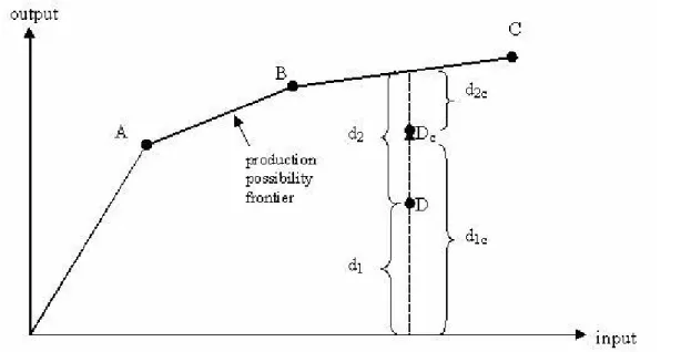
Figure 1 illustrates the basic idea behind a two-stage approach. In a simplified one output and one input DEA problem, A, B and C are found to be efficient, while D is an inefficient DMU. The output score for unit D equals (d1+d2)/d1, and is higher than

one. However, unit D inefficiency may be partly ascribed to a “harsh environment” – a number of perturbing environmental factors may imply that unit D produces less than the theoretical maximum, even if discretionary inputs are efficiently used. In our example, and if the environment for unit D was more favourable (e. g. similar to the sample average), then we would have observed Dc. In other words, unit D would have

produced more and would be nearer the production possibility. The environment corrected output score would be (d1c+d2c)/d1c, lower than (d1+d2)/d1, and closer to

unity.

11

See Ruggiero (2004) and Simar and Wilson (2004) for an overview.

12

Figure 1 – DEA and non-discretionary outputs

3.3. Non-discretionary inputs and bootstrap

The two-stage method has been criticised in so far as results are likely to be biased in small samples13. Note that a perturbation to an observation located on the DEA estimated frontier will shift that very same frontier. As a result, some DMUs will find themselves closer or further to the frontier, and their scores will change accordingly. In terms of equation (2), this means that the error term εi is serially correlated in a

complicated and unknown way. As the sample increases, this correlation disappears slowly in the DEA context. An additional source of bias comes from the fact that that non-discretionary variables zi in equation (2), are correlated to the error term εi. This

correlation derives from the correlation between non-discretionary inputs and the outputs (and most probably the other inputs), which were the ingredients to estimate the scores. Again, this last correlation also disappears asymptotically, but at a slow rate.

13

Thus, standard approaches to inference are usually not valid in small samples. To overcome this, Simar and Wilson (2004) propose an alternative estimation and inference procedures based on bootstrap methods.

Assume that the true efficiency score depends on the environmental variables, so that

, 1 )

,

( + ≥

= _{i i}

i ψ z β ε

δ (3)

where ψ is a smooth, continuous function and β a vector of parameters. εi is a

truncated normal random variable, distributed N(0,σ_ε2) with left-truncation at

) , (

1−ψ zi β .

The efficiency score that solves problem (1), δˆi, is then considered as an estimate for

i

δ , and this is the first stage in the procedure. The second stage is designed to assess

the influence of non-discretionary inputs on efficiency. Simar and Wilson (2004) propose two algorithms to achieve these two stages, which are presented below14.

The first algorithm involves the following steps:

[1] The computation of δˆ_{i for all n decision units by solving problem (1);}

[2] The estimation of equation (2) by maximum likelihood, considering it is a

truncated regression (and not a censored or Tobit regression).15 Denote by βˆ and σˆ _ε

the maximum likelihood estimates of β and σε.

[3] The computation of L bootstrap estimates for β and σε, in the following way:

For i = 1, ...., n draw εi from a normal distribution with variance σˆε2 and left

truncation at 1−z_iβˆ and compute δ_i* = z_iβˆ+ε_i

.

14

We implemented these algorithms in Matlab. Programmes and functions are available on request.

15

Estimate the truncated regression of δ_i* on zi by maximum likelihood, yielding

a bootstrap estimate ( * _ˆ*

, ˆ

ε σ

β ).

With a large number of bootstrap estimates (e.g. L=2000), it becomes possible to test hypotheses and to construct confidence intervals for β and σε. For example, suppose

that we want to determine the p-value for a given estimateβˆ₁ <0. This will be given

by the relative frequency of nonnegativeβˆ₁* bootstrap estimates.

It can be shown that the estimate δˆi is biased towards 1 in small samples. Simar and

Wilson (2004) second bootstrap procedure, “algorithm 2”, includes a parametric bootstrap in the first stage problem, so that bias-corrected estimates for the efficiency scores are produced. The production of these bias-corrected scores is done as follows:

[1] Compute δˆ_i for all n decision units by solving problem (1);

[2] Estimate equation (2) by maximum likelihood, considering it is a truncated

regression. Let βˆ and σˆ be the maximum likelihood estimates of _ε β and σε.

[3] Obtain L1 bootstrap estimates for each δi, the following way:

For i = 1, ...., n draw εi from a normal distribution with variance σˆε2 and left

truncation at 1−z_iβˆ and compute δ_i* = z_iβˆ+ε_i

.

Let i

i i

i y

y* _*

ˆ

δ δ

= , be a modified output measure.

Compute δˆi* by solving problem (1), where Y is replaced by

[

]

1 *

... yn

y

Y = . (But note that yiis not replaced byyi* in the left-hand side

of the first restriction of the problem.)

[4] Compute the bias-corrected output inefficiency estimator asδˆˆi =2.δˆi −δˆi*, where

*

ˆ

i

Once these first stage bias-corrected measures are produced, algorithm 2 continues by

replacing δˆi with δˆˆ in algorithm 1, from step 2 onwards. Following Simar and i

Wilson (2004), we set L1=100.

4. Empirical analysis

4.1. Data and indicators16

Education achievement, the output, is measured by the performance of 15-year-olds on the PISA reading, mathematics, problem solving, and science literacy scales in 2003. Note that the PISA programme was specially conceived to “monitor the outcomes of education systems in terms of student achievement on a regular basis and within an internationally accepted common framework”.17 Students from 40 countries were therefore evaluated with the same set of questions to be solved, in what constitutes the more recent exercise of this kind. In a parsimonious formulation, we use the four scores country average.18

As performance of 15-year olds is likely to depend on resources employed not only in one year, but also in previous years, we have taken time average values. We use two input measures:

- the total intended instruction time in public institutions in hours per year for the 12 to 14-year-olds, average for 2000-2002;

- the number of teachers per student in public and private institutions for secondary education, calculations based on full-time equivalents, average for 2000-2002.19 Table 2 summarises the key statistics for our selected data sample.

16

The data and the sources used in this paper are presented in the Annex.

17

See OECD (2004b, pp. 3).

18

The four results in the PISA report are highly correlated, with correlation coeficients ranging from 0.94 and 0.99.

19

Note that the number of observations used in the empirical analysis is lower than the number of countries that participated in the PISA, because some input variables are not available for some units in the sample.

Table 2 – Summary statistics of our data sample (25 countries)

Mean Standard

deviation

Minimum Maximum

PISA (2003) 490.5 41.4 374.6

(IND)

545.9 (FI) Teachers per 100

students (2000-02)

7.7 1.7 5.1

(KOR)

11.5 (PT) Hours per year in

school (2000-02)

946.5 121.2 740.9 (SW)

1274.0 (IND) Parent education

attainment (2001-02)

65.0 24.4 19.0 (THA)

94.0 (JP) GDP per capita, PPP

USD (2003)

22267.1 9327.9 3364.5 (IND)

37063.4 (NO)

Note: FI – Finland; IND – Indonesia; JP – Japan; KOR – Korea; NO – Norway; PT – Portugal; THA – Thailand.

Input measures such as the ones we are considering here, have been used by several other authors studying the relationship between educational inputs and outputs. Examples are Barro (2001), Hanushek and Kimko (2000), Hanushek and Luque (2003) and Kirjavainen and Loikkanen (1998).

We have considered the option of using education spending per student as an input. However, results would be hardly interpretable, as they would reflect both inefficiency and cost provision differences. For example, countries where teachers are better paid would tend to show up as inefficient, irrespective of the intrinsic performance of the education system. Moreover, results would also depend on the exchange rate used to convert expenses to the same units. Physical inputs and outputs have the important advantage of being comparable across countries without the need of any questionable transformation.

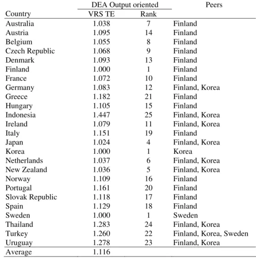
4.2. DEA efficiency results

Table 3 – Results for education efficiency (n=25)

2 inputs (teachers-students ratio, hours in school) and 1 output (PISA 2003 indicator)

DEA Output oriented

Country VRS TE Rank

Peers

Australia 1.038 7 Finland

Austria 1.095 14 Finland

Belgium 1.055 8 Finland

Czech Republic 1.068 9 Finland

Denmark 1.093 13 Finland

Finland 1.000 1 Finland

France 1.072 10 Finland

Germany 1.083 12 Finland, Korea

Greece 1.182 21 Finland

Hungary 1.105 15 Finland

Indonesia 1.447 25 Finland, Korea

Ireland 1.079 11 Finland, Korea

Italy 1.151 19 Finland

Japan 1.024 4 Finland, Korea

Korea 1.000 1 Korea

Netherlands 1.037 6 Finland, Korea

New Zealand 1.036 5 Finland, Korea

Norway 1.109 16 Finland

Portugal 1.161 20 Finland

Slovak Republic 1.118 17 Finland

Spain 1.129 18 Finland

Sweden 1.000 1 Sweden

Thailand 1.283 24 Finland, Korea

Turkey 1.260 22 Finland, Korea, Sweden

Uruguay 1.278 23 Finland, Korea

Average 1.116

Note: VRS TE – variable returns to scale technical efficiency.

It is possible to observe from Table 3 that three countries would be labelled as the most efficient ones with the standard DEA approach: Finland, Korea, and Sweden. Finland and Korea are located in the efficient frontier because they perform quite well in the PISA survey, getting respectively the first and the second position in the overall education performance index ranking. Sweden is also an above average performer concerning the output measure, using below average inputs. Another set of three countries is located on the opposite end – Thailand, Turkey and Uruguay. DEA analysis indicates that their output could be increased by more than 25 percent if they were to become efficient.20 On average and as a conservative estimate, countries could have increased their results by 11.6 percent using the same resources.

20

One can briefly compare this set of results with the ones reported by Afonso and St. Aubyn (2005) that addressed education efficiency using the PISA 2000 performance indicator and a similar set of inputs, even if, as mentioned by OECD (2004b), the PISA 2000 and the PISA 2003 are not fully comparable (the latter included an extra item). Interestingly, the countries located in the efficient frontier were Finland, Korea, Japan, and Sweden, essentially the same results as the ones we report.

4.3. Explaining inefficiency – the role of non-discretionary inputs

Using the DEA efficiency scores computed in the previous subsection, we now evaluate the importance of non-discretionary inputs. We present results both from Tobit regressions and bootstrap algorithms. Even if Tobit results are possibly biased, it is not clear that bootstrap estimates are necessarily more reliable. In fact, the latter are based on a set of assumptions that may be disputed. Equation (3) summarises some of these important assumptions concerning the data generation process and the perturbation term distribution. Taking the pros and cons of both methods into account, it seems sensible to apply both of them. If outcomes are comparable, this adds robustness and confidence to the results we are interested in.

In order to explain the efficiency scores, we regress them on GDP per capita, Y, and parents’ educational attainment, E, as follows21

i i i

i

β

β

β

ε

δ

in one of the inputs (Mexico has the lowest teachers per students ratio) or both of them (Brazil). Given the inputs allocated to education provision by these countries, their performance in the PISA index is not comparable to any other country with similar or inferior outcome and with lower inputs. Moreover, one has to note that Brazil and Mexico are among lowest PISA survey performers. Therefore, we do not consider these efficient by default DMUs in the main text. Their inclusion would not affect further results in any meaninful way. The interested reader may refer to the Appendix, where we present main results for the extended sample.

21

We first report in Table 4 results from the censored normal Tobit regressions for several alternative specifications of equation (4), namely including only one of the explanatory variables or taking logs of GDP per head.

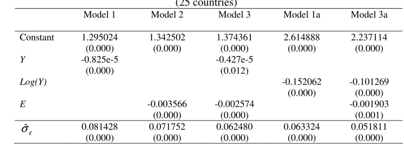
Table 4 – Censored normal Tobit results (25 countries)

Model 1 Model 2 Model 3 Model 1a Model 3a

Constant 1.295024 (0.000) 1.342502 (0.000) 1.374361 (0.000) 2.614888 (0.000) 2.237114 (0.000)

Y -0.825e-5

(0.000)

-0.427e-5 (0.012)

Log(Y) -0.152062

(0.000)

-0.101269 (0.000)

E -0.003566

(0.000) -0.002574 (0.000) -0.001903 (0.001) ε

σˆ 0.081428

(0.000) 0.071752 (0.000) 0.062480 (0.000) 0.063324 (0.000) 0.051811 (0.000)

Notes: Y – GDP per capita; E – Parental educational attainment. σˆ_ε – Estimated standard deviation of

ε. P- values in brackets.

Inefficiency in the education sector is strongly related to two variables that are, at least in the short to medium run, beyond the control of governments: the family economic background, proxied here by the country GDP per capita, and the education of parents. The estimated coefficients of both non-discretionary inputs are statistically significant and negatively related to the efficiency measure. For instance, an increase in parental education achievement reduces the efficiency score, implying that the relevant DMU moves closer to the theoretical production possibility frontier. Therefore, the better the level of parental education attainment, the higher the efficiency of secondary education provision in a given country. The same reasoning applies to the second non-discretionary input, with higher GDP per capita resulting in more efficiency.

are highly significant in statistical terms, with p-values equal or smaller than 0.001. That both factors may act in a separate way is suggested by identifying a group of countries in the sample that display high values for educational attainment in spite of being poorer than average (the Czech and Slovak Republics, Hungary, Korea) contrasting to richer countries with lower levels of adult education (Italy, Spain, Portugal).

Additionally, we also considered the ratio of public-to-total expenditure in secondary education as a non-discretionary input. However, this variable did not prove to be statistically significant, probably because most spending in this level of education is essentially public and high for most countries. We report those results in the Appendix, for a more reduced country sample due to data availability.

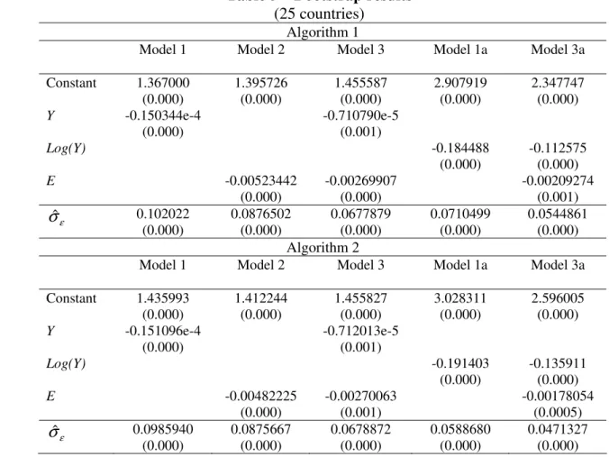
Table 5 – Bootstrap results (25 countries)

Algorithm 1

Model 1 Model 2 Model 3 Model 1a Model 3a

Constant 1.367000 (0.000) 1.395726 (0.000) 1.455587 (0.000) 2.907919 (0.000) 2.347747 (0.000)

Y -0.150344e-4 (0.000)

-0.710790e-5 (0.001)

Log(Y) -0.184488

(0.000)

-0.112575 (0.000)

E -0.00523442

(0.000) -0.00269907 (0.000) -0.00209274 (0.001) ε

σˆ 0.102022

(0.000) 0.0876502 (0.000) 0.0677879 (0.000) 0.0710499 (0.000) 0.0544861 (0.000) Algorithm 2

Model 1 Model 2 Model 3 Model 1a Model 3a

Constant 1.435993 (0.000) 1.412244 (0.000) 1.455827 (0.000) 3.028311 (0.000) 2.596005 (0.000)

Y -0.151096e-4 (0.000)

-0.712013e-5 (0.001)

Log(Y) -0.191403

(0.000)

-0.135911 (0.000)

E -0.00482225

(0.000) -0.00270063 (0.001) -0.00178054 (0.0005) ε

σˆ 0.0985940 (0.000) 0.0875667 (0.000) 0.0678872 (0.000) 0.0588680 (0.000) 0.0471327 (0.000)

Notes: Y – GDP per capita; E – Parental educational attainment. σˆ_ε – Estimated standard deviation of

ε; P- values in brackets.

In all three methods, it is apparent that Model 3a provides the best fit (as can be seen by the lower estimated standard deviation of ε). This is important and robust empirical evidence that efficiency in education depends both on a country’s wealth and on parents’ education levels. In a nutshell, students coming from poorer countries where adults’ education levels are low tend to under perform, so that results are further away from the efficiency frontier.

Equation (4) can be regarded as a decomposition of the output efficiency score into two distinct parts:

– the one that is the result of a country’s environment, and given by

i

i E

Y ₂

1

0

β

β

– the one that includes all other factors that have an influence on efficiency, including therefore inefficiencies associated with the education system itself, and given by εt.

The first column in Table 6 includes the bias corrected scores for Model 3a, the one with the best fit.22 Recall that algorithm 2 implies a bias correction after estimating output efficiency scores by solving program (1) and taking into account the correlation between these scores and the environmental variables. We also present score corrections for the two environmental variables. GDP and education attainment corrections were computed as the changes in scores by artificially considering that Y

and E varied to the sample average in each country. Fully corrected scores are estimates of output scores purged from environmental effects and result from the summation of the previous three columns.

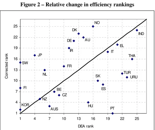
Comparing the ranks in the last column of Table 6, resulting from corrections for both bias and environmental variables, with the previously presented ranking from the standard DEA analysis (see Table 3 above), it is apparent that significant changes occurred. For instance, countries previously poorly ranked are now less far away from the production possibility frontier – this is the case of Portugal, Uruguay, Hungary, Turkey and Spain. On the other hand, some countries see a worsening in their relative position after taking into account environmental variables, namely Sweden, Japan, Denmark, Norway, Germany and Austria.

22

Table 6 – Corrected output efficiency scores (for Model 3a)

Bias corrected scores

(1)

GDP correction

(2)

Education attainment correction

(3)

Fully corrected scores (4)=(1)+(2)+(3)

Rank

Australia 1.047 0.037 -0.007 1.077 3

Austria 1.104 0.040 0.030 1.174 22

Belgium 1.063 0.033 -0.001 1.095 7

Czech Republic 1.083 -0.041 0.046 1.087 6

Denmark 1.108 0.048 0.028 1.184 23

Finland 1.037 0.027 0.035 1.100 8

France 1.082 0.028 0.005 1.115 14

Germany 1.104 0.029 0.037 1.170 21

Greece 1.191 -0.015 -0.010 1.167 20

Hungary 1.115 -0.058 0.024 1.082 4

Indonesia 1.528 -0.257 -0.075 1.196 24

Ireland 1.094 0.068 -0.002 1.159 19

Italy 1.160 0.026 -0.028 1.159 18

Japan 1.044 0.032 0.052 1.127 17

Korea 1.075 -0.030 0.023 1.068 2

Netherlands 1.066 0.038 0.009 1.112 13

New Zealand 1.068 -0.007 0.026 1.087 5

Norway 1.131 0.069 0.046 1.246 25

Portugal 1.172 -0.026 -0.080 1.067 1

Slovak Republic 1.131 -0.068 0.045 1.108 10

Spain 1.140 0.000 -0.035 1.105 9

Sweden 1.052 0.024 0.039 1.116 15

Thailand 1.348 -0.146 -0.082 1.120 16

Turkey 1.343 -0.162 -0.072 1.109 12

Uruguay 1.296 -0.134 -0.053 1.109 11

Average 1.143 -0.018 0.000 1.126

Additionally, by looking at GDP and education attainment corrections in Table 6, it is apparent that in some countries, environmental “harshness” essentially results from poor adult education, and less from low GDP per head, as in Spain and Portugal. In Hungary, the Czech Republic and Korea, on the other hand, lower than average GDP is offset by higher educational attainment. Finally, note that Indonesia, Thailand, Turkey and Uruguay are countries where both environmental variables strongly push down performance, as opposed to the Scandinavian countries or Japan.

Figure 2 – Relative change in efficiency rankings

FR

NL

PT NO

SW

ES

URU

HU

TUR JP

DK

DE AU

KOR FI

IR

IND

EL IT

THA

SK

AUS CZ BE

NZ

1 4 7 10 13 16 19 22 25

1 4 7 10 13 16 19 22 25

DEA rank

C

or

rec

ted r

ank

Note: AUS – Australia; AU – Austria; BE – Belgium; CZ - Czech Republic; DK – Denmark; FI – Finland; FR – France; DE – Germany; EL – Greece; HU – Hungary; IND – Indonesia; IR – Ireland; IT – Italy; JP – Japan; KOR – Korea; NL – Netherlands; NZ - New Zealand; NO – Norway; PT – Portugal; SK - Slovak Republic; ES – Spain; SW – Sweden; THA – Thailand; TUR – Turkey; URU - Uruguay.

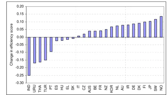
Figure 3 – Change in efficiency scores after correction

-/+: DMU moves closer (further away) to (from) the production frontier

-0.30 -0.25 -0.20 -0.15 -0.10 -0.05 0.00 0.05 0.10 0.15 0.20

IN

D

URU TH

A

TU

R

PT ES HU EL SK IT CZ

AU

S

BE FR NZ

KO

R

NL AU IR DE DK FI JP _SW NO

C

hange

in eff

ic

ienc

y

s

c

or

e

Note: see note to Figure 2 for country abbreviations.

Figure 3 essentially derives from the environmental harshness in each considered country. Indonesia, for example, being the poorest country in the sample and the second worst in terms of parents` educational attainment, is the place where environment is less favourable to student achievement. This implies that a bias corrected output score of 1.528 is reduced to 1.196, meaning that about 62.9 percent of measured inefficiency may be ascribed to exogenous factors. Norway is one opposite case – this is the richest country in the sample, and one where adults are more instructed. Taking this into account, leads to the highest fully corrected output score, 1.246. Note that Norwegian PISA average performance (492.23) was below other developed and comparable countries (e.g. Finland or Sweden).

5. Conclusion

standard DEA problem with countries as DMUs. Secondly, these scores were explained in a regression with the environmental variables as independent variables.

Results from the first-stage imply that inefficiencies may be quite high. On average and as a conservative estimate, countries could have increased their results by 11.6 percent using the same resources23, with a country like Indonesia displaying a waste of 44.7 percent.

The fact that a country is seen as far away from the efficiency frontier is not necessarily a result of inefficiencies engendered within the education system. Our second stage procedures show that GDP per head and parents’ educational attainment are highly and significantly correlated to output scores – a wealthier and more cultivated environment are important conditions for a better student performance. Moreover, it becomes possible to correct output scores by considering the harshness of the environment where the education system operates. Country rankings and output scores derived from this correction are substantially different from standard DEA results.

Non-discretionary outputs considered here cannot be changed in the short run. For example, parental educational attainment is essentially given when considering students performance in the coming year. However, contemporaneous educational and social policy will have an impact on future parents’ educational attainment. As the children of today are the parents of tomorrow, and considering that parental educational attainment is an important determinant of students’ outcomes, it results that policies oriented towards reducing present school dropout rates or increasing youth education length will positively affect the future efficiency of the educational system of given country.

Finally, note that we have applied both the usual DEA/Tobit procedure and two very recently proposed bootstrap algorithms. Results were strikingly similar with these three different estimation processes, which bring increased confidence to obtained conclusions.

23

Appendix – Additional Tobit and bootstrap results

Table A1 – Censored normal Tobit results (27 countries, includes Brazil and Mexico)

Model 1 Model 2 Model 3 Model 1a Model 3a

Constant 1.213629 (0.000) 1.265284 (0.000) 1.278989 (0.000) 2.178233 (0.000) 1.862711 (0.000)

Y -0.548e-5

(0.012)

-0.204e-5 (0.412)

Log(Y) -0.109971

(0.000)

-0.067701 (0.081)

E -0.002674

(0.000) -0.002192 (0.022) -0.001580 (0.095) ε

σˆ 0.106527

(0.000) 0.098319 (0.000) 0.096023 (0.000) 0.095875 (0.000) 0.090651 (0.000)

Notes: Y – GDP per capita; E – Parental educational attainment. σˆ_ε – Estimated standard deviation of

ε; P- values in brackets.

Table A2 – Censored normal Tobit results (21 countries)

Model 4 Model 5 Model 6 Model 7 Model 5a Model 7a Constant 1.483093 (0.000) 1.360996 (0.000) 1.605412 (0.000) 1.496527 (0.000) 2.626978 (0.000) 2.375158 (0.000)

Pub -0.417987 (0.241) -0.068827 (0.807) -0.286462 (0.236) -0.090810 (0.655) 0.148174 (0.515) 0.068794 (0.688)

Y -0.859e-5

(0.000)

-0.555e-5 (0.003)

Log(Y) -0.167262

(0.000)

-0.120034 (0.000)

E -0.003604

(0.000) -0.002742 (0.000) -0.002137 (0.000) ε

σˆ 0.109699 (0.000) 0.082045 (0.000) 0.073550 (0.000) 0.059098 (0.000) 0.063605 (0.000) 0.047561 (0.000)

Table A3 – Bootstrap results (27 countries, includes Brazil and Mexico)

Algorithm 1

Model 1 Model 2 Model 3 Model 1a Model 3a

Constant 1.29834 (0.000) 1.35914 (0.000) 1.49384 (0.000) 3.4082 (0.000) 2.52437 (0.001)

Y -0.22800e-4 (0.000)

-0.14238e-4 (0.001)

Log(Y) -0.25082

(0.000)

-0.13721 (0.0405)

E -0.0073074

(0.000) -0.0040814 (0.000) -0.00336 (0.048) ε

σˆ 0.17528

(0.000) 0.14757 (0.000) 0.10380 (0.000) 0.13497 (0.000) 0.12369 (0.000) Algorithm 2

Model 1 Model 2 Model 3 Model 1a Model 3a

Constant 1.35924 (0.000) 1.37764 (0.000) 1.40856 (0.000) 2.85792 (0.000) 2.38279 (0.000)

Y -0.12303e-4 (0.000)

-0.060890e-4 (0.002)

Log(Y) -0.17692

(0.000)

-0.11663 (0.000)

E -0.0045012

(0.0) -0.0026775 (0.0005) -0.0018025 (0.0025) ε

σˆ 0.09707

(0.000) 0.092488 (0.000) 0.071508 (0.000) 0.07532 (0.000) 0.064324 (0.000)

Notes: Y – GDP per capita; E – Parental educational attainment. σˆ_ε – Estimated standard deviation of

References

Afonso, A.; Schuknecht, L. and Tanzi, V. (2003). “Public Sector Efficiency: An International Comparison,” ECB Working Paper nº 242, forthcoming in Public

Choice.

Afonso, A. and St. Aubyn (2005). “Non-parametric Approaches to Education and Health Efficiency in OECD Countries,” forthcoming in Journal of Applied

Economics.

Barro, R. (2001). “Human Capital and Growth”, American Economic Review 91 (2), 12-17.

Barro, R. and Lee, J-W. (2001). ”Schooling Quality in a Cross-Section of Countries”,

Economica¸ 68 (272), 465-488.

Benhabib, J. and Spiegel, M. (1994), “The Role of Human Capital in Economic Development: Evidence from Aggregate Cross-Country Data”, Journal of Monetary

Economics,34 (2), 143-173.

Charnes, A.; Cooper, W. and Rhodes, E. (1978). “Measuring the efficiency of decision making units,” European Journal of Operational Research, 2 (6), 429–444.

Coelli, T.; Rao, P. and Battese, G. (1998). An Introduction to Efficiency and

Productivity Analysis. Kluwer, Boston.

De la Fuente, A. and Ciccone, A. (2002), Human capital in a global and

knowledge-based economy – final report, Brussels, European Commission, Directorate-General

for Employment and Social Affairs.

EC (2004). Public Finances in EMU - 2004. A report by the Commission services, SEC(2004) 761. Brussels.

Farrell, M. (1957). “The Measurement of Productive Efficiency,” Journal of the Royal

Statistical Society, Series A, 120, Part 3, 253-290.

Gupta, S. and Verhoeven, M. (2001). “The Efficiency of Government Expenditure – Experiences from Africa", Journal of Policy Modelling, 23, 433-467.

Hanushek, E. and Kimko, D. (2000). “Schooling, labor force quality, and economic growth”, American Economic Review, 90 (5), 1184-1208.

Hanushek, E. and Luque, J. (2003). “Efficiency and equity in schools around the world”, Economics of Education Review, 22, 481-502.

Kirjavainen T. and Loikkanen, H.A. (1998). “Efficiency differences of Finnish senior secondary schools: an application of DEA and Tobit analysis”. Economics of

Krueger, A. and Lindahl, M. (2001). “Education and growth: why and for whom?”

Journal of Economic Literature, 39, 1101-1136.

OECD (2002). Education at a Glance – OECD Indicators 2002, OECD, Paris.

OECD (2003a). Education at a Glance – OECD Indicators 2003, OECD, Paris.

OECD (2003b). “Enhancing the Cost Effectiveness of Public Spending,” in Economic

Outlook, vol. 2003/02, n. 74, December, OECD.

OECD (2004a). Education at a Glance – OECD Indicators 2004, OECD, Paris.

OECD (2004b). Learning for Tomorrow’s World – First Results from PISA 2003, OECD, Paris.

Pritchett, L. (2001). “Where Has All the Education Gone?”, World Bank Economic

Review, 15 (3), 367-391.

Ruggiero, J. (2004). “Performance evaluation when non-discretionary factors correlate with technical efficiency”, European Journal of Operational Research 159, 250–257.

Sianesi, B. and Van Reenen, J. (2003). “The Returns to Education: Macroeconomics”,

Journal of Economic Surveys, 17 (2), 157-200.

Simar, L. and Wilson, P. (2000). “A General Methodology for Bootstrapping in Nonparametric Frontier Models”, Journal of Applied Statistics, 27, 779-802.

Simar, L. and Wilson, P. (2004). “Estimation and Inference in Two-Stage, Semi-Parametric Models of Production Processes”, April, mimeo.

St. Aubyn, M. (2003). “Evaluating Efficiency in the Portuguese Education Sector”,

Economia, 26, 25-51.

Thanassoulis, E. (2001). Introduction to the Theory and Application of Data

Annex – Data and sources

Country PISA (2003)

1/

Hours per year in school, 2000-2002 2/ Teachers per 100 students, 2000-2002 3/ GDP per capita, 2003 (USD) 4/ Parental education attainment, 2001-2002 5/ Public-to-total expenditure ratio 2001-2002 6/

Australia 526.15 1023.7 8.0 29143. 4 61.1 84.6

Austria 498.35 1072.5 10.0 29972. 5 81.9 96.0

Belgium 517.59 1005.0 10.5 28396. 1 64.6 94.4

Brazil 379.84 800.0 5.5 7767. 2 57.3

Czech Republic 511.16 867.0 7.5 16448. 2 90.5 91.9

Denmark 499.65 860.0 7.8 31630. 2 80.5 97.9

Finland 545.90 807.0 7.3 27252. 2 84.7 99.3

France 509.34 1037.0 8.1 27327. 2 67.9 93.0

Germany 502.53 886.0 6.6 27608. 8 85.6 80.8

Greece 461.67 1064.0 10.1 19973. 2 59.4 91.6

Hungary 494.06 925.0 8.7 14572. 3 78.6 92.9

Iceland 501.57 821.9 na 30657. 3 61.0 95.2

Indonesia 374.55 1274.0 5.5 3364. 5 22.7 76.4

Ireland 505.54 896.3 7.0 36774. 8 63.7 95.7

Italy 474.31 1020.0 9.8 27049. 9 49.4 97.9

Japan 531.79 875.0 6.7 28162. 2 94.0 91.6

Korea 541.29 867.0 5.1 17908. 4 77.8 78.5

Mexico 393.56 1166.9 3.3 9136. 2 15.6 86.7

Netherlands 523.87 1066.9 6.1 29411. 8 69.9 94.8

New Zealand 524.68 952.6 6.1 21176. 9 79.6 na

Norway 492.23 826.8 9.6 37063. 4 90.8 99.2

Poland 492.81 na 6.8 11622. 9 47.9 na

Portugal 470.29 881.7 11.5 18443. 5 20.0 99.9

Russian Federation 469.61 989.0 8.9 9195. 2 na na Slovak Republic 488.49 886.3 7.4 13468. 7 90.3 98.1

Spain 483.75 907.2 8.6 22264. 45.3 93.1

Sweden 509.50 740.9 7.3 26655. 5 86.8 99.9

Switzerland 514.99 887.0 na 30186. 1 87.3 86.9

Thailand 422.73 1167.0 5.6 7580. 3 19.0 97.8

Tunisia 365.70 890.0 4.6 7082. 9 na 100.0

Turkey 426.54 841.3 5.7 6749. 3 24.7 na

United States 486.67 na 6.5 37352. 1 88.5 91.5

Uruguay 426.35 913.0 6.9 8279. 9 35.1 93.5

Mean 480.82 942.5 7.4 21202.3 63.9 92.8

Minimum 365.70 740.9 3.3 3364.5 15.6 76.4

Maximum 545.90 1274.0 11.5 37352.1 94.0 100.0

Standard deviation 48.87 122.0 1.9 10168.7 24.6 6.5

Observations 33 31 31 33 31 28 na – not available.

1/ Average of performance of 15-year-olds on the PISA reading, mathematics, problem solving and science literacy scales, 2003. Source: OECD (2004b).

2/ Total intended instruction time in public institutions in hours per year for 12 to 14-year-olds, average for 2000-2002. Source: OECD (2002, 2003a, 2004a, Table D1.1).

3/ Students per teaching staff in public and private institutions, secondary education, calculations based on full-time equivalents, average for 2000-2002. Source: OECD (2002, 2003a, 2004a, Table D2.2).

4/ PPP GDP and population in 2003. Source: World Development Indicators Database, September 2003. 5/ Population that has attained at least upper secondary education, aged 35-44, average for 2001-2002. OECD(2003a, Table A1.2, 2004a, Table A2.2).

European Central Bank working paper series

For a complete list of Working Papers published by the ECB, please visit the ECB’s website (http://www.ecb.int)

448 “Price-setting behaviour in Belgium: what can be learned from an ad hoc survey?” by L. Aucremanne and M. Druant, March 2005.

449 “Consumer price behaviour in Italy: evidence from micro CPI data” by G. Veronese, S. Fabiani, A. Gattulli and R. Sabbatini, March 2005.

450 “Using mean reversion as a measure of persistence” by D. Dias and C. R. Marques, March 2005.

451 “Breaks in the mean of inflation: how they happen and what to do with them” by S. Corvoisier and B. Mojon, March 2005.

452 “Stocks, bonds, money markets and exchange rates: measuring international financial transmission” by M. Ehrmann, M. Fratzscher and R. Rigobon, March 2005.

453 “Does product market competition reduce inflation? Evidence from EU countries and sectors” by M. Przybyla and M. Roma, March 2005.

454 “European women: why do(n’t) they work?” by V. Genre, R. G. Salvador and A. Lamo, March 2005.

455 “Central bank transparency and private information in a dynamic macroeconomic model” by J. G. Pearlman, March 2005.

456 “The French block of the ESCB multi-country model” by F. Boissay and J.-P. Villetelle, March 2005.

457 “Transparency, disclosure and the Federal Reserve” by M. Ehrmann and M. Fratzscher, March 2005.

458 “Money demand and macroeconomic stability revisited” by A. Schabert and C. Stoltenberg, March 2005.

459 “Capital flows and the US ‘New Economy’: consumption smoothing and risk exposure” by M. Miller, O. Castrén and L. Zhang, March 2005.

460 “Part-time work in EU countries: labour market mobility, entry and exit” by H. Buddelmeyer, G. Mourre and M. Ward, March 2005.

461 “Do decreasing hazard functions for price changes make any sense?” by L. J. Álvarez, P. Burriel and I. Hernando, March 2005.

462 “Time-dependent versus state-dependent pricing: a panel data approach to the determinants of Belgian consumer price changes” by L. Aucremanne and E. Dhyne, March 2005.

463 “Break in the mean and persistence of inflation: a sectoral analysis of French CPI” by L. Bilke, March 2005.

464 “The price-setting behavior of Austrian firms: some survey evidence” by C. Kwapil, J. Baumgartner and J. Scharler, March 2005.

465 “Determinants and consequences of the unification of dual-class shares” by A. Pajuste, March 2005.

466 “Regulated and services’ prices and inflation persistence” by P. Lünnemann and T. Y. Mathä, April 2005.

468 “Endogeneities of optimum currency areas: what brings countries sharing a single currency closer together?” by P. De Grauwe and F. P. Mongelli, April 2005.

469 “Money and prices in models of bounded rationality in high inflation economies” by A. Marcet and J. P. Nicolini, April 2005.

470 “Structural filters for monetary analysis: the inflationary movements of money in the euro area” by A. Bruggeman, G. Camba-Méndez, B. Fischer and J. Sousa, April 2005.

471 “Real wages and local unemployment in the euro area” by A. Sanz de Galdeano and J. Turunen, April 2005.

472 “Yield curve prediction for the strategic investor” by C. Bernadell, J. Coche and K. Nyholm, April 2005.

473 “Fiscal consolidations in the Central and Eastern European countries” by A. Afonso, C. Nickel and P. Rother, April 2005.

474 “Calvo pricing and imperfect common knowledge: a forward looking model of rational inflation inertia” by K. P. Nimark, April 2005.

475 “Monetary policy analysis with potentially misspecified models” by M. Del Negroand F. Schorfheide, April 2005.

476 “Monetary policy with judgment: forecast targeting” by L. E. O. Svensson, April 2005.

477 “Parameter misspecification and robust monetary policy rules” by C. E. Walsh, April 2005.

478 “The conquest of U.S. inflation: learning and robustness to model uncertainty” by T. Cogley and T. J. Sargent, April 2005.

479 “The performance and robustness of interest-rate rules in models of the euro area” by R. Adalid, G. Coenen, P. McAdam and S. Siviero, April 2005.

480 “Insurance policies for monetary policy in the euro area” by K. Küster and V. Wieland, April 2005.

481 “Output and inflation responses to credit shocks: are there threshold effects in the euro area?” by A. Calzaand J. Sousa, April 2005.

482 “Forecasting macroeconomic variables for the new member states of the European Union” by A. Banerjee, M. Marcellino and I. Masten, May 2005.

483 “Money supply and the implementation of interest rate targets” by A. Schabert, May 2005.

484 “Fiscal federalism and public inputs provision: vertical externalities matter” by D. Martínez-López, May 2005.

486 “What drives productivity growth in the new EU member states? The case of Poland” by M. Kolasa, May 2005.

487 “Computing second-order-accurate solutions for rational expectation models using linear solution methods” by G. Lombardo and A. Sutherland, May 2005.

488 “Communication and decision-making by central bank committees: different strategies, same effectiveness?” by M. Ehrmann and M. Fratzscher, May 2005.

489 “Persistence and nominal inertia in a generalized Taylor economy: how longer contracts dominate shorter contracts” by H. Dixon and E. Kara, May 2005.

490 “Unions, wage setting and monetary policy uncertainty” by H. P. Grüner, B. Hayo and C. Hefeker, June 2005.

491 “On the fit and forecasting performance of New-Keynesian models” by M. Del Negro, F. Schorfheide, F. Smets and R. Wouters, June 2005.

492 “Experimental evidence on the persistence of output and inflation” by K. Adam, June 2005.

493 “Optimal research in financial markets with heterogeneous private information: a rational expectations model” by K. Tinn, June 2005.