Numerical solution of curved pipes submitted to in-plane loading conditions

(1)

Numerical solution of curved pipes submitted to in-plane loading conditions

E.M.M. Fonseca

a,

_{, F.J.M.Q. de Melo}

b a_{Department of Applied Mechanics, Polytechnic Institute of Braganc}

-a, Portugal b_{Department of Mechanical Engineering, University of Aveiro, Portugal}

a r t i c l e

i n f o

Article history:

Received 31 October 2008 Accepted 18 September 2009

Keywords: Curved pipe In-plane loading Linear analysis Polynomial function

a b s t r a c t

An alternative formulation to current meshes dealing with finite shell elements is presented to solve the problem of stress analysis of curved pipes subjected to in-plane bending forces. The solution is based on finite curved elements, where displacements are defined from a total set of trigonometric functions or a fifth-order polynomial, combined with Fourier series. Global shell displacements are achieved through the one associated with curved arch bending and the other referred to the toroidal thin-walled shell distortion. Beam-type displacement and in-plane rotation are uncoupled and separately formulated, using trigonometric shape functions, as in Timoshenko or Mindlin beam theory. To build up the solution, a simple deformation model was adopted, based on the semi-membrane concept of the doubly curved shells behaviour. Several studies are presented and compared with experimental and numerical analyses reported by other authors.

1. Introduction

Curved pipes are structural elements of essential applications in the transport of fluids in chemical processes, or energy generation plants, eventually at elevated pressure or temperature. These piping elements exhibit complex deformation fields given their toroidal geometry and the multiplicity of configurations of external loads. This is a technical matter under investigation for a long time by researchers working in this field; von Ka´rmań[1] published the first solution for the problem of characterization of stress analysis in pipe bends subjected to in-plane bending. Essentially, the solution was based on the Rayleigh–Ritz method, but its application field was quite restricted, as only curved pipes with no end restrains were considered in the problem; in fact even the inclusion of tangent terminations could not be included in the problem. Vigness [2] generalized the solution presented by Ka´rmań[1] and presented an experimental procedure to verify the derived bending equations, Cheng and Thailer[3]reduced the problem of in-plane bending to two coupled ordinary differential equations that could be integrated without simplifying assump-tions. More recently Thomson [4] worked with an analytical formulation using in the displacement field a development with doubly defined trigonometric series functions and performed many experimental studies. O¨ ry and Wilczek [5] presented an economical method based on transfer matrix techniques to define the stress and deformation calculation. Ohtsubo and Watanabe[6] presented what could be really named as the first finite curved

pipe element. In this finite ring element the displacement field was defined as a combination of second-order Hermitian func-tions and trigonometric funcfunc-tions in the longitudinal and circumferential directions, respectively. Bathe and Almeida [7] formulated a pipe elbow element using a cubic displacement interpolation based on finite-element method with the ovaliza-tion phenomena contribuovaliza-tion. The work of these two authors included the useful internal pressure effect, an essential para-meter to achieve realistic and safe designs as well as a non-linear material behaviour.

Some relevant contributions in this area have been published recently by Melo and Castro [8,9] using short and straight elements as an approach to curved pipes with simple first-degree polynomials. Orynyak [10] used specific analytical methods developed to perform elastic end effects for pipe bends. As they present remarkable ovalization when subjected to bending moments, they are vulnerable components when they are subjected to loads during the transport of chemically aggressive fluids, a situation potentially favourable to corrosion under tension. These structural elements are much more flexible when compared with straight pipes subjected to the same forces. The stress field from the same bending moment appears now intensified for curved pipes, as a consequence of the distortion section due to the ovalization and warping phenomena. Many experiments and theories have been presented by Findlay and Spence [11] and Wilczek [12] to demonstrate and explain the flexibility and stress field of a curved pipe compared with elastic beam theory. A computational model for the stress analysis of tubular structures is presented in this paper. The work is based on shell displacement field and elastic theory and a finite curved pipe element with two nodes is presented. The displacement field is Contents lists available atScienceDirect

journal homepage:www.elsevier.com/locate/tws

Thin-Walled Structures

(2)

based on trigonometric functions for curved arch displacements and the development of Fourier series to model warping and ovalization of tubular sections. This element will be compared with results obtained with other element based on high-order polynomial functions for curved arch displacements, such as the equations developed by Fonseca et al. [13,14]. This element presents good accuracy for displacement and stress ﬁelds resulting from in-plane bending under generalized loads. With this element the behaviour of curved pipe end effects is also analyzed. The stress state calculation at any transverse section is easy, given the simplicity of the involved algorithms. The main advantage is associated with the generation of simple meshes with low number of elements, remarkable economy in degrees of freedom and in computational time.

2. Assumptions

The deformation field of a finite pipe element refers to membrane strain and curvature variation. Definition of the geometric parameters are follows: the arch length s, the mean radius of curvatureR, the thicknessh, the mean section radius of the piperand the central angle

a

. For any point of the shell surface w is the transverse shell displacement,u the longitudinal shell displacement and v the meridional shell displacement. Fig. 1 shows the essential geometric parameters deﬁning the two-node ﬁnite curved pipe element.

The basic equations governing the behaviour of thin shells were derived by Love[15]. The following assumptions, referred to by Fonseca et al.[14,16], were considered in the present analysis:

(a) The radius of curvature is assumed much larger than the section radius. This means that the ‘pipe bore term’ (R+rcos

y

) may be approximated toR.

(b) A semi-membrane deformation model is adopted and neglects bending stiffness along the longitudinal direction of toroidal shells, but considers meridional bending resulting from ovalization.

(c) The shell is considered thin and inextensible along the meridional direction

y

, which means that the hoop strain

e

yy=0.

e

yy¼wþ @v

@

y

ð1Þ

The arch is thin, that is,rZh. Typically the thickness should be less than a tenth of the mean pipe radius.

The deformation model considers that the pipe undergoes a semi-membrane strain field. The strain field is given by the following equations, also used by Melo and Castro[8,9], Fl ügge [17]and Kitching[18]:

e

ss

gs

y

w

yy 8 > <

> :

9 > =

> ;

¼ @ @s

sin

y

R cos

y

R 1

r

@ @

y

@ @s 0

0 1

r2

@ @

y

1 r2

@2

@

y

2

6 6 6 6 6 6 6 4

3

7 7 7 7 7 7 7 5

u v w 8 > <

> :

9 > =

> ;

ð2Þ

where

ess

is the longitudinal membrane strain,

gs

ythe shear strain and

w

yyis the meridional curvature from ovalization.

3. Displacement field for a two-node curved pipe element

The deformation model for arch elements follows the Love– Kirchhoff assumptions, with inextensibility for the mean curved line. A set of differential relations defines the displacement and strain fields for slender arch theory by On_ate~ _[19]_{. The} displace-ment field for curved pipe eledisplace-ments is calculated from the mean line of each arch considered as a rigid beam element:Uis the tangential displacement, W the transverse displacement and

j

the rotation inzdirection represented inFig. 2.

When finite pipe elements have in-plane displacements, a formulation based on trigonometric functions (TF) is used and four parameters are necessary to define the displacement field.U can be approximated by the following function:

UðsÞ¼a1cos s

R þa2sin s

R þa3cos 2 s R

þa4sin 2 s R

ð3Þ

Fig. 1.Geometric parameters for the ﬁnite pipe element.

Nomenclature

an constants to be determined of the ovalization dis-placements

[B] deformation matrix

bn constants to be determined of the warping displace-ments

[D] elasticity matrix

E elastic modulus

{Fn} applied nodal forces

h thickness of the pipe

[K] elementary stiffness matrix Myy meridional stress

N shape function

Ny number of trigonometric terms used in Fourier

expansions

Nss longitudinal stress

Nsy shear stress

R mean curvature radius

r mean section pipe radius

s pipe arch length or longitudinal direction [T] transpose matrix for global system

U tangential displacement

W transverse displacement

a

central pipe angle

gs

y shear strain

{

d

} nodal displacement vector

ess

longitudinal strain

y

meridional direction

n

Poisson’s ratio

j

rotation

(3)

The transverse displacement refers to the inextensibility for arch mean curved line and can be calculated as

WðsÞ¼ R dU

ds ¼a1sin s

R a2cos s

R þa32 sin 2 s R

a42 cos 2 s R

ð4Þ

For the rotation ﬁeld a linear polynomial is deﬁned from an uncoupled equation:

j

_ðsÞ¼a5þa6S ð5Þ

The unknown parameters {ai} are determined by imposing boundary conditions according to the curved referential, Fig. 2, for the nodesiandjconsidered, resulting in the system equations to be solved:

Ui Wi

j

i Uj Wj

j

j 8 > > > > > > > > > < > > > > > > > > > : 9 > > > > > > > > > = > > > > > > > > > ; ¼

1 0 1 0 0 0

0 1 0 2 0 0

0 0 0 0 1 0

cosð

a

Þ sinð

a

Þ cosð2

a

Þ sinð2

a

Þ 0 0 sinð

a

Þ cosð

a

Þ 2 sinð2

a

Þ 2 cosð2

a

Þ 0 0

0 0 0 0 1 L

2 6 6 6 6 6 6 6 6 4 3 7 7 7 7 7 7 7 7 5 a1 a2 a3 a4 a5 a6 8 > > > > > > > > > < > > > > > > > > > : 9 > > > > > > > > > = > > > > > > > > > ;

ð6Þ

From those conditions, a new set of shape functionsNi¼1;...;4and

Ni¼1;...;4 are determined and the generic local displacements for

in-plane ﬁnite-element formulation are given from the following equations:

UðsÞ¼ ðUiN1þUjN2Þ þ ðWiN3þWjN4Þ ð7Þ

WðsÞ¼ RððUiN10 þUjN20 Þ þ ðWiN30 þWjN40ÞÞ ð8Þ

j

ðsÞ¼

j

iNiþ

j

jNj ð9Þ

An equivalent solution could be developed using a ﬁfth-order polynomial (5P) [13,14]. Conclusions about the performance of such alternatives are discussed in advance.

The distortion displacement field concerns ovalization and meridional displacements for transverse cross-sections[4]. These displacements are defined from simple first-order polynomial functionsNiandNjfor the longitudinal directions, combined with Fourier expansions for the meridional direction

y

.

The surface displacement in the radial direction resulting from ovalization is expressed by the equation

wðs;yÞ¼

X

nZ2

anicosn

y

! Niþ

X

nZ2

anjcosn

y

!

Nj ð10Þ

As a consequence of the assumed inextensibility of the perimeter of the transverse section (assumption c) the meridional displacement due to ovalization is calculated from the following equation:

vðs;yÞ¼

X

nZ2 ani

n sinn

y

!

Niþ

X

nZ2 anj

n sinn

y

!

Nj ð11Þ

The coefﬁcientsaniand anjare constants to be determined and included in the Fourier expansions of ovalization displacements for in-plane bending. Finally, the longitudinal displacement due to warping of the pipe section is deﬁned from the following equation:

uðs;yÞ¼

X

nZ2

bnicosn

y

! Niþ

X

nZ2

bnjcosn

y

!

Nj ð12Þ

The parametersbniandbnjare also functions of developed series resulting from warping in-plane displacements.

The ﬁnite shell element displacement resulting from a displacement superposition of a rigid arch element and a complete Fourier expansion for ovalization and warping terms is presented as follows:

u v w 8 > < > : 9 > = > ; local ¼

N1 N3 Nircosy 0 cos_{|fflfflffl{zfflfflffl}}ny

Ni j

RN10 siny RN30 siny 0 sinny

n

|fflfflfflfflffl{zfflfflfflfflffl}

Ni 0 j

RN10 cosy RN30 cosy 0 cosny

|fflfflffl{zfflfflffl}

Ni 0 j

2 6 6 6 6 6 6 6 6 6 6 6 6 4

j N2 N4 Njrcosy 0 cos_{|fflfflffl{zfflfflffl}}ny

Nj

j RN20 siny RN40 siny 0

sinny n

|fflfflfflfflffl{zfflfflfflfflffl}

Nj 0

j RN20 cosy RN40 cosy 0 cos_{|fflfflffl{zfflfflffl}}ny

=Nj 0

3 7 7 7 7 7 7 7 7 7 5 Ui Wi

j

i ani bni Uj Wj

jj

anj bnj 8 > > > > > > > > > > > > > > > > > > > > > > > > < > > > > > > > > > > > > > > > > > > > > > > > > : 9 > > > > > > > > > > > > > > > > > > > > > > > > = > > > > > > > > > > > > > > > > > > > > > > > > ;

ð13Þ

The developed element has two nodal sections and a total of 38 degrees of freedom, 19 for each section (2 translations, 1 in-plane rotation, 8 terms for ovalization and 8 terms for warping).

α

X Y

Wi Ui Wj

Uj

ϕi

ϕj R

i j

Fy (i or j)

Fx (i or j) Mz (i or j)

s

(4)

Application of the principle of virtual work leads to the system of algebraic equations of the problem solution. Having solved the system of algebraic equations, the displacement ﬁeld is obtained for all nodes of the structure. The matrix force–displacement equation for this ﬁnite pipe element model is

½Kf

d

g ¼ fFng ð14Þ

where {

d

} is a nodal unknown displacement vector and {Fn} is the applied nodal forces acting on sectionsiandj. This force vector is formed by terms involving longitudinal and transverse forces, bending moments or terms related to the Fourier expansions for the ovalization and warping displacements. The element stiffness matrix [K] is calculated from the following equation:

½K ¼ ½Tð Z

s

½BT½D½BdSÞ½TT ð15Þ

wheredS=r ds d

y

, [T] is the transpose matrix for global system, [B] results from the derivative of shape functions for the ﬁnite pipe element and [D] is the elasticity matrix, dependent on the elastic modulusE, the pipe thicknesshand Poisson’s ratiov:

½D ¼ Eh

1

n

2 0 0

0 Eh

2ð1þ

n

Þ 0

0 0 Eh3

12ð1

n

2_Þ 2

6 6 6 6 6 6 6 4

3

7 7 7 7 7 7 7 5

ð16Þ

Due to the uncoupled formulation of the displacementWand the section rotation

j

in the two-node curved beam element in discussion, it is necessary that a different type of integration should be used along variables. This expedient avoids the element locking, a numerical drawback associated with the contribution of shear terms in the stiffness matrix when exact integrations are used. The use of selective reduced integration only for shear terms has shown a remarkable improvement in the numerical behaviour of pipe elements, a procedure used by Melo and Castro[8]and Prathap[20]. In the formulation of the pipe element formulated here, a reduced Gauss integration was carried out along variables while an exact one was used along the circumferential direction

y

. In detail, the stiffness terms resulting from the beam shear deformation were calculated using one-point Gauss integration, while all the remaining stiffness terms were calculated with two-point Gauss integration. The total number of degrees of freedom for this element is 2(3+2Ny), where Ny is the number of trigonometric terms used in Fourier expansions equal 8 terms.

Finally, the stress ﬁeld is then deﬁned for each element in the following form:

Nss

Nsy Myy 8 > <

> :

9 > =

> ;

¼ ½D

e

ss

gs

y

w

yy 8 > <

> :

9 > =

> ;

ð17Þ

whereNssis the longitudinal membrane stress,Nsythe shear stress andMyythe meridional bending stress.

4. Case studies

To assess the accuracy of the element in discussion, some examples are analyzed in this section. In some of them, external loads are conventional in the project of piping systems (as for example, the pure bending moment) while in others, less

42.66°

R1110 1.2

M = 1.256E6N.mm

Ø340 Thick or Thin Flanges

Thick or Thin Flanges M = 1,256E6N.mm

Fig. 3.Geometry of a curved pipe loaded by a concentrated moment with end restraints.

-24 -20 -16 -12 -8 -4 0 4 8 12 16

0

Degrees

Nss [N/mm

2]

30 60 90 120 150 180

Melo and Castro Wilczek (matrix method) Wilczek (experimental) 5P 5elements

TF 5elements 5P 10elements TF 10elements

Fig. 4.Longitudinal stress for a curved pipe with rigid ﬂanges.

-40 -20 0 20 40 60

0

Degrees

Nss [N/mm

2]

30 60 90 120 150 180

Melo and Castro

Wilczek (matrix method)

Wilczek (experimental)

5P 5elements

TF 5elements

5P 10elements

TF 10elements

(5)

conventional external loads were included in the examples. Apparently, they are not of interest in the design of piping systems and in fact they are avoided, like the example of edge-concentrated loads. Their inclusion in this work is associated with a more elaborated solution needed for stress analysis, and hence presented here. All forces and moments considered in Eq. (14) must be referred to the global system of elements, except constriction forces due to ovalization or warping displacements.

4.1. Curved pipe under in-plane pure bending

The next example refers to a curved pipe with end restraints subjected to a uniform bending moment, as shown inFig. 3. This

example was taken from the work of Wilczek [12], who

investigated the stress analysis of curved pipes using the transfer matrix method and experimental tests. This example was also analyzed by Melo and Castro [8] with a ﬁnite pipe element developed by them. Here only one half of the pipe bend was analyzed due to geometry and loading symmetries. The results refer to the transverse section equidistant from the pipe ends, either with rigid or thin ﬂanges, as shown inFig. 3.

Figs. 4 and 5present the longitudinal stresses of a curved pipe

under pure bending moment, using rigid or thin ﬂanges. Results obtained with this formulation based on trigonometric functions (TFs) for beam terms using a ﬁfth-order polynomial (5P), with different meshes, are compared with the results produced by Melo and Castro [8]and Wilczek [12]. Longitudinal stresses are represented along the half span (0–1801) of the transverse section.

4.2. Curved pipe loaded with a pair of concentrated forces

Fig. 6presents the same test specimen represented inFig. 3,

but now loaded with a bending moment resulting from a pair of concentrated forces, acting on a thin ﬂange. The ﬂange of the

42.66°

R 11₁₀

1.2

Ø340

Thick Flange

Thin Flange

F = 3676.5N

F = 3676.5N s/L

Fig. 6.Geometry of a curved pipe loaded with a pair of concentrated forces.

-40 -30 -20 -10 0 10 20 30

0

Degrees

Nss [N/mm

2]

30 60 90 120 150 180

Melo and Castro

Wilczek (matrix method) Wilczek (experimental)

5P 5elements

TF 5elements 5P 15elements

TF 15elements

Fig. 7.Longitudinal stress for a curved pipe loaded with a pair of concentrated forces (s/L=0.1).

-25 -20 -15 -10 -5 0 5 10 15

0

Degrees

Nss [N/mm

2]

30 60 90 120 150 180

Melo and Castro

5P 5elements

TF 5elements

5P 15elements

TF 15elements

Fig. 8. Longitudinal stress for a curved pipe loaded with a pair of concentrated forces (s/L=0.5).

-40 -30 -20 -10 0 10 20 30

0

Degrees

Nss [N/mm

2]

Melo and Castro

5P 5elements

TF 5elements

5P 15elements TF 15elements

30 60 90 120 150 180

(6)

built-in edge is considered rigid. Thin ﬂanges do not ovalize and the warp forces are considered like as referred to by Melo and Castro [8]. For a pair of concentrated longitudinal forces, of opposed senses, acting like an in-plane bending moment, the force vector must be obtained with the following expression:

fFngT¼ f0;0;2Fr

|fflfflfflfflfflfflfflffl{zfflfflfflfflfflfflfflffl}

beam

;0;0;0;0;0;0;0;0

|fflfflfflfflfflfflfflfflfflfflfflfflfflffl{zfflfflfflfflfflfflfflfflfflfflfflfflfflffl}

ovalization

;0;2F;0;2F;0;2F;0;2F |fflfflfflfflfflfflfflfflfflfflfflfflfflfflfflfflfflfflfflffl{zfflfflfflfflfflfflfflfflfflfflfflfflfflfflfflfflfflfflfflffl}

warping

gT

ð18Þ

Figs. 7–9present the longitudinal membrane stress for three

different sections positions along the longitudinal direction of the

curved pipe. The present results using two different mesh reﬁnements are compared with corresponding data from other references included in the ﬁgures.

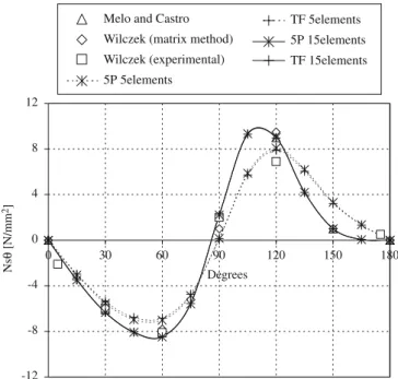
Figs. 10–12present the shear membrane stresses for the different

longitudinal positions of the curved pipe. There is a good approximation even when a coarse mesh is used when compared with the results calculated by Wilczek[12]and Melo and Castro[8].

5. Conclusion

The present method is a simple and economic tool for the determination of stress fields in curved pipes using a special formulation of finite elements. Despite the relatively low number of degrees of freedom, the results show that the elements are accurate and easy to manipulate. Pre- and post-processing operations with this pipe element suggest the possibility of its use in small personal computers; in fact the finite-element mesh set-up refers to the definition of a curved line, where each node contains information for beam displacements and transverse section distortion. The obtained values of stress distribution along transverse sections showed a good agreement with corresponding results from other analyses. This element solves the generalized in-plane loading problems using two distinct alternative formula-tions for the displacement field, even in cases of complex loads acting on the pipe ends. The solution presented here has performed well even with coarse element meshes. The proposed method appears as a simple and easy-to-handle alternative to the use of current meshes dealing with finite shell elements, which not only demand more expensive pre-processing programs but also generate a higher number of unknowns.

References

[1] von Ka´rmań Th. Über die Formänderung d ünnwaindiger R öhre, insbesondere federnder Ausgleichr öhre. Zeitschrift des Vereines Deutscher Ingenieure 1911;55:1889–95.

[2] Vigness I. Elastic properties of curved tubes. Transactions of the ASME 1943;65:105–20.

[3] Cheng DH, Thailer MJ. On the bending of curved circular tubes. ASME Journal of Engineering Industry 1970;92(1) [ser.B 62–66].

-8 -6 -4 -2 0 2 4 6 8 10

0

Degrees

Ns

θ

[N/mm

2]

30 60 90 120 150 180

Melo and Castro

5P 5elements

TF 5elements

5P 15elements

TF 15elements

Fig. 10.Shear membrane stress for a curved pipe loaded with a pair of concentrated forces (s/L=0.1).

-8 -6 -4 -2 0 2 4 6 8

0

Degrees

Ns

θ

[N/mm

2]

30 60 90 120 150 180

Melo and Castro

5P 5elements

TF 5elements

5P 15elements TF 15elements

Fig. 11.Shear membrane stress for a curved pipe loaded with a pair of concentrated forces (s/L=0.5).

-12 -8 -4 0 4 8 12

0

Degrees

Ns

θ

[N/mm

2]

Melo and Castro Wilczek (matrix method)

5P 5elements

TF 5elements 5P 15elements

TF 15elements

30 60 90 120 150 180

(7)

[4] Thomson G. The inﬂuence of end constraints on pipe bends. PhD thesis, University of Strathclyde, Scotland, UK, 1980.

[5] O¨ ry H, Wilczek E. Stress and stiffness calculation of thin-walled curved pipes with realistic boundary conditions being loaded in the plane of curvature. International Journal of Pressure Vessels and Piping 1983;12:167–89. [6] Ohtsubo H, Watanabe O. Stress analysis of pipe bends by ring elements.

Journal of Pressure Vesssel Technology 1978;100:112–21.

[7] Bathe KJ, Almeida CA. A simple and effective pipe elbow element—pressure

stiffening effects. Journal of Applied Mechanics 1982;49:914–6.

[8] Melo FJMQ, Castro PMST. A reduced integration Mindlin beam element for linear elastic stress analysis of curved pipes under generalized in-plane loading. Computers and Structures 1992;43(4):787–94.

[9] Melo FJMQ, Castro PMST. The linear elastic stress analysis of curved pipes under generalized loads using a reduced integration ﬁnite ring element. Journal of Strain Analysis 1997;32(1):47–59.

[10] Orynyak IV. First approximation to elastic analysis of end-effects in pipe bends. International Journal of Pressure Vessels and Piping 2002;79:157–64. [11] Findlay GE, Spence J. In-plane bending of a large 90

%

o smooth bend. Journal of Strain Analysis 1966;1(4):290.

[12] Wilczek E. Statische Berechnung Eines Rohrkr ¨ummers mit Realen Randbedingungen. PhD thesis, Technischen Hochschule Aachen, Aachen, 1984.

[13] Fonseca EMM, Melo FJMQ, Oliveira CAM. The thermal and mechanical behaviour of structural steel piping systems. International Journal of Pressure Vessels and Piping 2005;82(2):145–53.

[14] Fonseca EMM, de Melo FJMQ, Oliveira CAM. Numerical analysis of piping elbows for in-plane bending and internal pressure. Thin-Walled Structures 2006;44:393–8.

[15] Love AEH. A treatise on the mathematical theory of elasticity. New York; 1944.

[16] Fonseca EMM, Melo FJMQ, Oliveira CAM. Determination of ﬂexibility factors on curved pipes with end restraints using a semi-analytic formu-lation. International Journal of Pressure Vessels and Piping 2002;79(12): 829–40.

[17] Fl ¨ugge W. Thin elastic shells, 2nd ed. Berlin: Springer; 1973.

[18] Kitching R. Smooth and mitred pipe bends. In: Gill SS, editor. The stress analysis of pressure vessels and pressure vessels components. Oxford: Pergamon Press; 1970 [Chapter 7].

[19] On˜ate E. Ca´lculo de Estructuras por el Me´todo de Elementos Finitos [in spanish, Structure Calculation using the Finite Element Method]. CIMNE edition, The Polythecnic University of Calaunia, 1992.