Digital Underwater Acoustic Communication Simulator

Universidade Autónoma de Lisboa

Departamento de Ciências e Tecnologias

Licenciatura em Engenharia Eletrónica e de Telecomunicações

Digital Underwater Acoustic Communication Simulator

Paper prepared by: David Sampaio - 2015 João Aleixo - 20150576 Sérgio Silva - 20160626

Unidade Curricular: Laboratório de Projeto Under the guidance of

Professor Doutor Mário Marques da Silva

i

Abstract

The Underwater acoustic communication is still a relatively new term both for students and for researchers. The two thirds of water that cover our planet continuous to have much to give, and the rising interest on the oceans will continue on the future. As the interest increase, increases too the will of the researchers in use the oceans as a means, a channel of communication that can be effectively used. As we will see, this is a challenge task, fist because electromagnetic waves cannot be used in the underwater environment, so insisted of electromagnetic waves this study is turned to the study of acoustic waves and its performance on the underwater environment. As will related in this paper there are various challenges that will be explained one by one. In the first chapter there will be discussed the theories and the underwater channel properties, as well the MIMO system that implies the use of more than one antenna to transmit and receive in a way that the signal we want to send reaches de destination with substantial performance. The last chapter will be more focused on the simulation of that communication channel and its results will become clearer.

ii

Index

2. Underwater Acoustic Channel Characteristics ... 7

2.1. Introduction... 7 2.2. Speed of sound...7 2.3. Attenuation... 10 2.4. Multipath ... 10 2.6. Doppler Effect ... 11 2.7. Propagation Loss ... 12 2.7.1. Frequency-Dependent Absorption... 12

2.7.2. Geometric Spreading Loss... 12

2.7.3. Scattering Loss ... 12

2.8. Noise and External Interference ... 13

3. Underwater Acoustic Communication System ... 14

3.1. Introduction ... 14

3.2. Small Scale and Large Scale ... 14

3.3. The different components of the Fading ... 16

3.3.1. Large Scale... 17

3.3.2. Path Loss ... 17

3.3.3. Shadowing effect ... 18

3.3.4. Small Scale Fading ... 18

3.3.5. Flat Fading ... 18

3.3.6. Frequency Selective Fading... 18

3.3.7. Fast fading ... 18

iii

3.4. Waves behave, Refractions and reflections in the (UWA) ... 20

3.5. Multipath rays choose ... 21

3.6. OFDM and SC-FDE ... 21

3.7. Digital Modulation Techniques QPSK ... 23

4. MIMO Systems ... 25

4.1. Introduction ... 25

4.2. MIMO ... 26

4.3. Massive MIMO ... 27

4.4. MIMO Systems benefices ... 31

4.4.1. Diversity Techniques ... 31

4.4.2. Gain diversity ... 33

4.4.3. Spatial multiplexing gain ... 35

4.5. Distance Between MIMO Antennas ... 36

5. Simulations and Analysis of Results ... 39

5.1. Performance Results ... 39

5.2. Results without Correlation between Antenna Elements... 40

5.3. Results with Correlation between Antenna Elements... 46

6. Conclusions ... 52

6.1. Conclusion ... 52

6.2. Dificulties ... 54

iv

List of Figures

Figure 3 MATLAB creating an uncorrelated plot Figure 4MATLAB with 4 diverse plots

Figure 5 Shows the beave (speed) of the acoustic waves when exposed to Salinit y, pressure and temperature

Figure 6 Multiple paths refractions behave in shallow water

Figure 7 Multiple paths of acoustic rays in deeper water environment Figure 8 The components of the Rice Model

Figure 9 A scheme that collects all the existing types of fading Figure 10: Acoustic wave dispersion scheme in a not deeper water Figure 11 Multiple paths of acoustic rays in deeper water environment Figure 12 QPSK modulation Scheme

Figure 13 - A typical T=2 and R=2 MIMO system

Figure 14 - Massive MIMO using beamforming credits to 5g.co.uk

Figure 15 - Passible massive MIMO antenna configuration, credits 5g.co.uk

Figure 16 - Possible Massive MIMO used in underwater ambient using acoustic transmission

Figure 17 - Gain diversity in transmission Figure 18 Gain diversity in reception

Figure 19 - Spatial Multiplexing gain system

Figure 20 What is expected to be when there is a distance of 50cm between antennas. Figure 21 What we propose to be our real distance between antenas, with correlation. Figure 22 - BER results with one transmitting antenna and one receiving antenna (T=1, R=1) in SISO

Figure 23 - BER Results with 2 antennas of transmission and 4 antennas of reception. (T=2, R=4), MIMO

Figure 24 . BER results using 8 antennas of transmission and 2 antennas of reception (T=8, R=2), MIMO

v

Figure 26 BER results with 16 transmitting antennas and 64 receiving antennas, (T=16, R=64), a typical m-MIMO configuration

Figure 27 BER Results with 8 emission antennas and 2 receive antennas (T=8, R=2), with correlation coefficient of 0.3

Figure 28 BER results with 8 transmitting antennas and 2 receiving antennas (T=8, R=2), in m-MIMO with a correlation coefficient of 0.5

Figure 29 BER results with 8 transmitting antennas and 2 receiving antennas (T=8, R=2), in an m-MIMO typical configuration with a correlation coefficient of 0.65

Figure 30: BER results with 8 transmitting antennas and 2 receiving antennas (T=8, R=2), in a m-MIMO configuration with a correlation coefficient of 0.8

Figure 31: A plot that combines a majority of non-correlated and correlated techniques in order to have a bigger picture

Figure 32 BER results of IB-DFE without correlation with 8 transmitting antennas and 8 receiving antennas (T=8, R=8)

vi

List of Abbreviations

UWA Underwater Acoustic BER Bit Error Rate

DFE Decision Feedback Equalizer EGC Equal Gain Combiner

FDE Frequency Domain Equalization

IB-DFE Iterative-Block Decision Feedback Equalization MFB Matched Filter Bound

MIMO Multiple Input Multiple Output MISO Multiple Input Single Output MMSE Minimum Mean Square Error MRC Maximum Ratio Combiner

OFDM Orthogonal Frequency Division Multiplexing PSU Practical Salinity Unit

QPSK Quadrature Phase Shift Keying

SC-FDE Single-Carrier Frequency Domain Equalization SISO Single Input Single Output

SIMO Single Input Multiple Output SOFAR Sound Fixing and Ranging

ZF Zero Forcing

ISI Inter Symbol Interference EMW electromagnetic waves PAPR peak-to-average power ratio SM spatial multiplexing

MU-MIMO user systems

BS base station

CSI channel state information DSC Deep sound channel

vii FFT Fast Fourier Transformer IFFT Inverse fast Fourier transformer QPSK Quadrature Phase Shift Keying TDD Time division Duplex

1

Project Plan

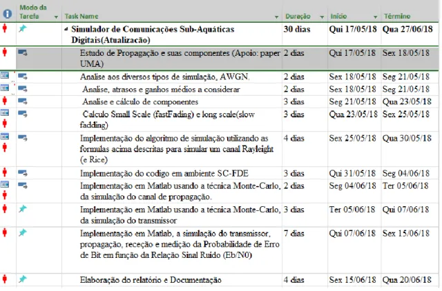
The first step in creating this project was by beginning to make the plan of the activities and to distribute the work through the 3 elements of the group like showed in Figure 1

At first there were only 2 elements of the Group. Sergio and João. This is the first MS Project plan created.

Figure 1 MS Project Print from early planning (march)

At the beginning our main issue was to study the underwater channel impairments, study the small scale and large scale and chose the algorithm to simulate our communications channel.

2

Figure 2 MS Project from a planning in May

At this point David has joined our group, and there was a need to elaborate another MS Project like pictured in Figure 2. At this point the group had figured that the Small scale was the model to use, and began study on the Rice fading distribution and Rayleigh fading distribution. At this point the first part of our paper was already developed, which correspond to the chapter 2 “Underwater Acoustic Channel Characteristics ”. From this point (end of May) until the end of august the main focus was spent in elaborating the results section. The results section corresponds the part of choosing the algorithm and the transmission techniques, as well as making the plots, commenting the plots, analyzing the results and elaborating this paper.

3

Project Requirements

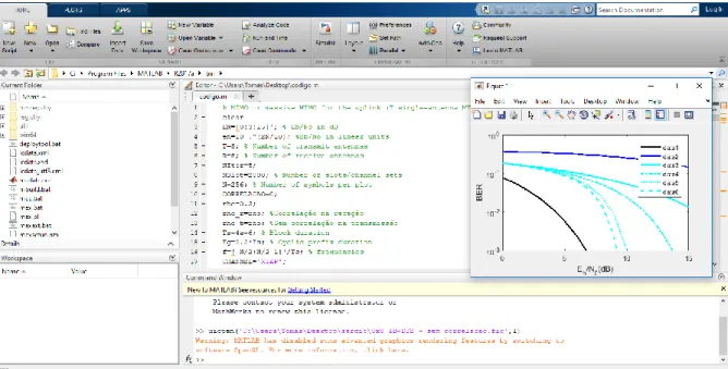
The basic project requirements include search for specific software. The choose was MATLAB, like pictured in Figure 3. With this software and the specific algorithm, we could simulate the channel characteristics as well design plots and more.

Search for specific literature, which was scarce since the topic underwater acoustic communications is still relatively new and unstudied.

Figure 3 MATLAB creating an uncorrelated plot

Project Initiation

Like said before the project initiated by characterizing the channel impairments and choosing which system (Small or large scale) we would use.

The project initiation includes installation of MATLAB, and some specific literature that was researched in the project requirements. The book that catalyst and make the group start the project was the Book “OFDM for Underwater Acoustic

4

Project execution

The project execution consists mainly in running the correct algorithm and plotting the necessary results as well as commenting them. For that an exhaustive search both on online papers as well online thesis and other articles was made, that could help the group on creating this paper. The algorithm was presented us from our tutor. The group only had to alter some parts of the code in order to change some parameters that made possible the creation of the desired plots. Only after that the rest of the work could be concluded.

5 1. Introduction

The planet earth is constituted to its surface by 2/3 of water and has always been throughout the history of humanity a target of great interest and curiosity. Aristotle in 400 BC stated that the sound could be both heard underwater as well as outside. In 1490 Leonardo da Vinci wrote "If you stop a ship and put one end of a long tube in the sea water and the other end in the ear you can hear other ships that are at a long distance." In 1826 Charles Sturm and Daniel Colladon made the first reliable measure of the speed of sound in water in Lake Geneva in Switzerland. But it was not until the beginning of the 20th century that the first practical application was seen. The headlamp vessels were fitted with a sound emitter that circulated in the water. Ships battling a thunderstorm and seeing the lighthouse ship could perceive the distance to these lighthouse ships because of the difference between sound propagation by air and water. In the first great war (1914-1918) considerable progress was made in underwater acoustic communication mainly in echo "echo ranging" communication in which the sound was emitted either at extremely low frequencies or high frequencies, the sonar principle that were put into practice by Constantin and Chilowski [1] But only during World War II did the step to understand how the sound propagated in the water. At that time, it was understood that the refraction of the sound in the water occurred due to 3 properties of the aquatic environme nt : Temperature, salinity and pressure as shown in Figure 5

In 1945, at the end of the second major war, the North American Navy created the first underwater telephone that allowed communication between ships and submarines using Suppressed Carrier Single Side Band Amplitude Modulation also known as SSB that operated at a frequency of 8.0875 Hz. frequency because the frequency of the quartz crystal is 16,175 Hz, that is, 2x bandwidth.

There are 3 main motivations that we established before the elaborations of this paper. The first one being the intensive study of the characteristics of the underwater channel and all its elements. The second to get into a conclusion whereas is it viable or not to make an acoustic underwater communications system, and on third point if possibly create a simulation where we can compare the diverse results. That part is well explained in chapter 4 where the diversity properties of the MIMO system open doors to compare

6

the various diversity transmission techniques. And on the conclusion, all our results, thoughts and experiences are shared.

7

2. Underwater Acoustic Channel Characteristics

2.1.Introduction

Given the complexity of underwater acoustic medium and the low propagation speed of sound in water, the underwater acoustic channel is commonly regarded as one of the most challenging channels for communication. As there will be shown later, the group have bet on the MIMO underwater system in an effort to have better performance results. Aldo the speed of the underwater acoustic waves reaches speeds greater than in the air, passing the speed of sound, that speed is not generally equal to all marine environments. In shallow waters the speed will have one value, and in deep waters the speed will have other value (higher in most cases)[2]. Underwater communications are getting more attention in the last years, and only when we have a fully understanding of the underwater acoustic channel characteristics, can we gradually make the underwater acoustic transmission system to match with the real marine environment, so as to achieve better performance.

2.2.Speed of sound

The extremely slow propagation speed of sound through seawater is an important factor that differentiates it from electromagnetic propagation. The speed of sound in water depends on the water properties of temperature, salinity and pressure; illustrative plots of the three parameters as functions of water depth are shown in Figure 5. A typical speed of sound in water near the ocean surface is about 1520 𝑚/𝑠, which is more than 4 times faster than the speed of sound in air, but five orders of magnitude smaller than the speed of light.

8

Figure 5 Shows the beave (speed) of the acoustic waves when exposed to Salinity, pressure and temperature

At the surface of the water the speed of sound travels at a speed of 1520m / s which corresponds to 5472km / h, while in air the sound travels at a speed of 331m / s corresponding to a speed of 1192 km / h, speed of the light responsible for the propagation velocity of the electromagnetic waves circulates at a

1079252848km / h. When we use acoustic waves as a means of underwater communication, we understand that propagation velocity is going to be the first dilemma we will encounter[3]

The speed of sound in water grows with increasing water temperature, increasing salinit y and increasing depth. Approximately, the sound speed increases 4.0 𝑚/𝑠 for water temperature rising 1°𝐶. When salinity increases one PSU, the sound speed in water increases to 1.4 𝑚/𝑠. As the depth of water (therefore also the pressure) increases to 1 km, the sound speed increases roughly to 17 𝑚/𝑠.

9

Figure 6 Multiple paths refractions behave in shallow water

Figure 7 Multiple paths of acoustic rays in deeper water environment

According to Snell's law, a ray of sound bends toward the direction of low propagation speed. In shallow water, the sound speed is usually constant throughout the water column. The acoustic signal usually propagates along straight lines, as illustrated in Figure 6. The sound speed profile of deep-water channels diversifies the sound propagation paths. In particular, notice that there is a minimal sound speed at a particular water depth (named the channel axis) between the permanent thermocline layer and the deep isothermal layer. For an acoustic signal transmitted at the channel axis, a ray of sound will be bent downward when propagating to the permanent thermocline layer and bent upward when

10

propagating to the isothermal layer, thus being trapped within the two layers without interacting with the sea surface and bottom, as illustrated in Figure 7

This type of channel is called the deep sound channel (DSC), and the corresponding propagation is called SOFAR[4]. An interesting phenomenon of SOFAR propagation is that a path traveling a longer distance could have a shorter travel time. Due to the refraction caused by inhomogeneous sound speed, there exist both shadow zones and convergence zones in the acoustic field, where a shadow zone denotes an area which cannot be penetrated by direct sound paths, and a convergence zone denotes in area which is insonified intensively by a bundle of sound paths.

2.3.Attenuation

A typical characteristic on an acoustic channel is that the overall path loss depends on the frequency. In an underwater acoustic channel, the attenuation is set by the absorption loss and the spreading loss. The first one corresponds to the conversion of acoustic energy in heat, and it depends on the chemical properties of sea water. The absorption loss in sea water is frequency dependent [17].

In conclusion, the underwater absorption, when dealing with high-frequency signals has strong impact on the attenuation as they traverse the channel. The spreading loss, on other hand, refers to the spreading of energy over an expanding volume as signals propagate in the medium. It can be cylindrical, typically seen in shallow waters, or it can be spherical, mostly observed in deep waters.

2.4.Multipath

For multipath, the effects of multipath in shallow waters are mainly reflections in the surface, in the bottom and in possible objects that are in the scene. These reflections are the responsible for causing multiple arrivals to the receiver. It can be presented generally

ℎ(𝑡) = ∑ ℎ_𝑝𝛿(𝑡 − 𝜏_𝑝) 𝑃

𝑝=0

Where ℎ_𝑝 are the paths amplitudes and can be considered as a low pass filter due to channel attenuation properties. Multiple arrivals are the roots of fading since interfere nce of different paths can be constructive or destructive. Simplified models for the fading are commonly accepted in UWA channels, like Rayleigh or Rician.

11 2.5.Time Varying Multipath

An acoustic wave transmission can reach a certain point through multiple paths. For shallow water transmissions, where the distance is much greater than the depth, the reflections of the wave at the bottom and at the surface generate delayed copies of the transmitted signal. For deep water transmissions, the reflections at the bottom and the surface can be disregarded, and variations in the velocity profile of the sound also produce multiple paths. In addition, multiple courses may vary over time. The two main factors that cause these variations are: changes in the environment and the Doppler effect.

2.6. Doppler Effect

The temporal variation of the multipath is a challenging problem when working with the underwater acoustic channel and the Doppler effect is its main cause in the underwater environment.

Doppler effect is of extreme importance when dealing with mult icarrier communicatio ns. Little frequency variations can cause an important degradation in performance. Usually, frequency shifts are corrected with hardware via resampling due to the cost of the operation, while Doppler spectrum estimation can be done in a low-complexity manner once having the sampled signals.

Doppler shift, this effect, caused by the relative motion of two bodies, is of special importance in underwater channels. The low speed of sound, which is about 𝑐 =

1500 𝑚/𝑠 and varying slightly with the speed prole, is the principal cause of this effect. Waves and currents make both the transmitter and receiver elements to be in continuous movement even if they are still on the bottom.

Doppler spectrum, the models behind Rayleigh or Rician fading assume that many waves arrive each with its own random angle of arrival (thus with its own Doppler shift), which is uniformly distributed within [0: : : 2𝜋], independently of other waves. This allows to compute a probability density function of the frequency of incoming waves. If we look at the Rayleigh fading channel in the time domain we find that the autocorrelation functio n of a specific tap (single arrival) is a first order Bessel function which depends of the maximum Doppler spread.

12 2.7. Propagation Loss

There are three primary mechanisms of energy loss during the propagation of acoustic waves in: absorptive loss, geometric spreading and scattering loss.

2.7.1. Frequency-Dependent Absorption

During propagation, wave energy may be converted to other forms and absorbed by the medium. The absorptive energy loss is directly controlled by the material imperfec t io n for the type of physical wave propagating through it. For EM waves, the imperfection is the electric conductivity of seawater. For acoustic waves, this material imperfection is the inelasticity, which converts the wave energy into heat.

2.7.2. Geometric Spreading Loss

Geometric spreading is the local power loss of a propagating acoustic wave due to energy conservation. When an acoustic impulse propagates away from its source with longer and longer distance, the wave front occupies larger and larger surface area. Hence, the wave energy in each unit surface (also called energy flow) becomes less and less. For the spherical wave generated by a point source, the power loss caused by geometric spreading is proportional to the square of the distance. On the other hand, the cylindrical waves generated by a very long line source, the power loss caused by geometric spreading is proportional to the distance.

2.7.3. Scattering Loss

Scattering is a general physical process in which the incident wave is reflected by irregular surfaces in many different directions. The sound scattering in underwater environments can be attributed to the nonuniformities in the water column and interactions of acoustic waves with nonideal sea surfaces and bottoms. Obstacles in the water column include point targets such as fish and plankton, and scattering volumes such as fish bubble clouds. The corresponding scattering loss depends on the acoustic wavelength and target size. In particular, the scattering loss increases as the acoustic wavelength decreases. The scattering property of sea surface and bottom is mainly determined by the interface roughness. High interface roughness induces large spatial energy dispersion. The roughness of sea surface is due to the capillary waves caused by wind, the amplitude of which ranges from centimeters to meters (e.g., swells).

13

In real scenarios, the two types of spreading processes coexist. The types of spreading losses occur when the acoustic wave interacts with the surface of the sea and the clouds of bubbles. In addition, wind-generated waves become mobile reflectors of the acoustic waves, thus introducing energy dispersion not only in the spatial domain, but also in the frequency domain.

2.8. Noise and External Interference

Noise is used to denote a signal that distorts the desired ones. Depending on applicatio ns, underwater acoustic noise consists of different components. Specific to the underwater acoustic communication system, the acoustic noise can be grouped into two categories: ambient noise and external interference.

Ambient noise is one kind of background noise which comes from a myriad of sources. The common sources of ambient noise in water include volcanic and seismic activit ies, turbulence, surface shipping and industrial activities, weather processes such as wind -generated waves and rain, and thermal noise [266]. Due to the multiple sources, ambient noise can be approximated, as Gaussian, but it is not white. The level of underwater ambient noise may have large fluctuations upon a change with time, location or depth. For short-range acoustic communication, the level of ambient noise may be well below the desired signal. For long-range or covert acoustic communication, the noise level would be a limiting factor for communication performance.

External interference is an interfering signal which is recognizable in the received signal. Corresponding sources include marine animals, ice cracking, and acoustic systems working in the same environment. Sonar operations could occasionally happen at the same time with communications, creating an external interference which is highly structured [422]. Relative to ambient noise, external interferences are neither Gaussian nor white. The presence of this kind of noises may cause highly dynamic link error rate or even link outage.

14

3. Underwater Acoustic Communication System

The ever-increasing demand for bandwidth, efficiency, spatial diversity and performance of underwater acoustic (UWA) communication has opened doors for the use of Multi-Input Multi-Output (MIMO) as will be referred in the next chapter.

Underwater communication is predominantly by acoustic waves and characterized as time-varying, multipath environment. However, the attenuation and delay associated with the acoustic channel mitigates the range and data rate available. A Channel simula tor were required to support the deployment of these study which relies on the characterization of the underwater acoustic channel. Acoustic communication is suitable at low frequency. Thus, modeling of multipath propagation especially Doppler Effect plays an important role. In this chapter there will be discussed some important questions that must be answered to develop a reliable underwater acoustic communication system, such as the choose between small scale and large scale, a briefly definition of the various types of fading and the reflections and refractions of the underwater acoustic rays behave, block transmission techniques (SC-FDE and OFDM) [5] and a briefly explanation of the QPSK that have been used in this study to simulate the characterization of the communication channel. Finally, there will be presented an example of a MIMO system where will be calculated the number on antennas and deduced the space between them.

3.2. Small Scale and Large Scale

Based on estimations and studies there was a need to choose between the use of a Small Scale or a Large-Scale fading model on underwater acoustic communications. Large scale fading or as sometimes referred “Shadowing” are related to large distances effects so, its affect appears clearly in case of the displacement of either the Transmitter or the Receiver. The clearest example for this case is the RF reception for a Car or a moving vehicle where the signal is influenced by Multipath phenomena where the transmitted signal is received from more than one path, and so the Large-scale fading uses a normal log distribution to calculate the fading of the ray elements. However Small-scale fading is concerned about very small changes in the position of Transmitter or receiver in order of the wavelengt h

15

as this affect greatly the received frequency thanks to the doppler effect. Therefore, the small-scale fading uses a rice distribution.

Rice Distribution is a model for radio propagation anomaly or interference caused by partial cancellation of a radio signal by itself. The signal arrives at the receiver by different paths, and we can assume that it suffers of multipath interference), and at least one of the paths is changing, lengthening or shortening. Rice fading happens when one of the paths, typically a line of sight signal or some strong reflection signals, is much stronger than the others and the amplitude gains are characterized by a Rician distribut io n. In the rice Model when there is no possibility of a line-of-sight signal, there is a need to use the Rayleigh fading. Basically, the Rician distribution degenerates to a Rayleigh distribution when the dominant component fades away[6].

We can assume than that the Rice Model is when exists a Line-of- sight signal component and when that is not possible meaning there is no line-of-sight there is a need to add the Rayleigh fading component like is indicated in the Figure 8

Figure 8 The components of the Rice Model

Rayleigh fading is the specialized model for fading when there is no line-of-sight signal, and is sometimes considered as a special case of the more generalized concept of Rician fading. In Rayleigh fading, the amplitude gain is characterized by a Rayleigh distribut io n. The requirement that there be many scatters present means that Rayleigh fading can be a useful model in heavily built-up city centers where there is no line of sight between the transmitter and receiver and many buildings and other objects attenuate, reflect, refract, and diffract the signal.

The study presented here focus in acoustic underwater communications and after this small introduction of the small scale and large-scale systems there is a sense to use the small scale, first because the small scale is a model where there is a Line-of-sight signal, and there are not large variations or large objects in the line of sight path, and it is more indicated to large areas where there are not obstacles between the transmitter and the

16

receiver, and that is exactly what happens in the underwater environment. When the dominant component fades away thanks to the reflect, refract, and diffract of the acoustic waves, Rician distribution degenerates to a Rayleigh fading distribution.[7]

3.3. The different components of the Fading

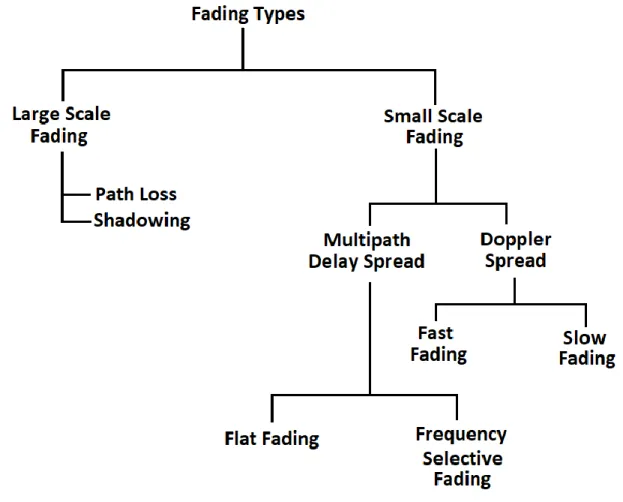
Fading is generally a signal loss either in amplitude or phase due to sudden changes in Channel response. The time variation of received signal power due to changes in transmission medium or paths is known as fading. fading depends on atmospheric conditions such as rainfall, lightening etc. In the underwater environments fading can be worsen if meteorological conditions such as storms, thunderstorms or waves. Generally fading depends on obstacles over the path which are varying with respect to time. These obstacles create complex transmission effects to the transmitted signal. Figure 9 shows all types of fading possible that will be explained latter.

17

Fading signals occur due to reflections from ground and surrounding buildings as well as scattered signals from trees, people and towers present in the large area. In the underwater environment, algae fish, the sand plankton and others may create scattering in the acoustic signals.

There exist different channel impairments and position of transmitter/receiver and

therefore there are 2 types of fading in wireless communication system.

Large Scale Fading: Includes path loss and shadowing effects.

Small Scale Fading: is divided into two categories. multipath delay spread and doppler spread. The multipath delay spread is further divided into flat fading and frequency selective fading. Doppler spread is divided into fast fading and slow fading.

3.3.1. Large Scale

Large scale fading happens when an obstacle comes in between transmitter and receiver. This interference causes sa large amount of signal strength reduction.

3.3.2. Path Loss

The free space path loss can be expressed as follows.

𝑃_𝑡/𝑃_𝑟 = {(4 × 𝜋 × 𝑑)^2/𝜆^2 } = (4 × 𝜋 × 𝑓 × 𝑑)^2/𝑐^2 Where,

Pt = Transmit power Pr = Receive power λ = wavelength

d = distance between transmitting and receiving antenna c = speed of light i.e. 3 x 108

From the equation it implies that transmitted signal attenuates over distance as the signal is being spread over larger and larger area from transmit end towards receive end.

18 3.3.3. Shadowing effect

Shadowing is the effect that the received signal power fluctuates due to objects obstructing the propagation path between transmitter and receiver. These fluctuations are experienced on local-mean powers, that is, short-term averages to remove fluctuat io ns due to multipath fading.

3.3.4. Small Scale Fading

Small scale fading is when rapid fluctuations of received signal strength over very short distance and short time period.

Based on multipath delay spread there are two types of small scale fading Flat fading and frequency selective fading. These multipath fading types depend on propagation environment.

3.3.5. Flat Fading

The wireless channel is said to be flat fading if it has constant gain and linear phase response over a bandwidth which is greater than the bandwidth of the transmitted signal. In this type of fading all the frequency components of the received signal fluctuate in same proportions simultaneously. It is also known as non-selective fading.

The effect of flat fading is seen as decrease in SNR. These flat fading channels are known as amplitude varying channels or narrowband channels. [8]

3.3.6. Frequency Selective Fading

It affects different spectral components of a radio signal with different amplitudes. Hence the name selective fading.

Based on doppler spread there are two types of fading: fast fading and slow fading. These doppler spread fading types depend on mobile speed i.e. speed of receiver with respect to transmitter.

3.3.7. Fast fading

Fast fading is represented by rapid fluctuations of signal over small areas. When the signals arrive from all the directions in the plane, fast fading will be observed for all

19

directions of motion. Fast fading occurs when channel impulse response changes very rapidly within the symbol duration, and have the following characteristics

-High doppler spread

-Symbol period > Coherence time -Signal Variation < Channel variation

This parameter results into frequency dispersion or time selective fading due to doppler spreading. Fast fading is result of reflections of local objects and motion of objects relative to those objects. The received signal in fast fading, is the sum of numerous signals which are reflected from various surfaces. This signal is the sum or difference of mult ip le signals which can be

constructive or destructive based on relative phase shift between them. Phase relationships depend on speed of motion, frequency of transmission and relative path lengths.

Fast fading distorts the shape of the baseband pulse. This distortion is linear and creates ISI (Inter Symbol Interference). Adaptive equalization reduces ISI by removing linear distortion induced by channel.

3.3.8. Slow Fading

Slow fading is result of shadowing by buildings, hills, mountains and other objects over the path. And is characterized by the following details.

-Low Doppler Spread

-Symbol period <<Coherence Time -Signal Variation >> Channel Variation

Slow fading results in a loss of SNR. Error correction coding and receiver diversity techniques are used to overcome effects of slow fading.

20

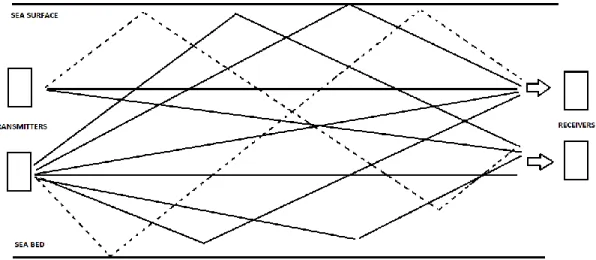
3.4.Waves behave, Refractions and reflections in the (UWA)

Figure 10: Acoustic wave dispersion scheme in a not deeper water

Different than the electromagnetic waves (EMW) the acoustic waves have a differe nt behavior in un underwater environments, and can even change as deeper they go. On surface water with low temperature, the behavior of the rays of sound, usually follows a pattern of constant propagation as if it were of refractions as shown in Figure 10. But as the depth increases and the sounds propagate in the several layers rays of sound follow a behavior described according to the Law of Snell's, in which a ray of sound curves in the direction of the low speed of propagation, the lower the speed of propagation of the sound, the greater curvature will have the radius of sound. As the variation of the speed of sound also varies the curvature of the sound ray. In an acoustic sound signal, transmitted at 1000 meters depth, where the velocity is smaller, will make a downward curvature when transmitted to the Permanent thermocline layer and curvature upwards when transmitted to the Deep isothermal layer as is shown Figure 11.

21

Figure 11 Multiple paths of acoustic rays in deeper water environment

3.5.Multipath rays choose

After figuring out which model should be used (in this study Small Scale) and its details, there was much debate at how much rays should be simulated. The authors started using a small number of rays in the beginning of the work, but the results were ambiguous, and so there was urge to increase the number of rays. The authors opted later to use 20 rays with uncorrelated and correlated Rice fading on the simulation to be able to make a channel more pessimist in rays path and between the transmitter and receiver and also in post processing of the data. The channel is considered invariant throughout the transmission period of a block, although it varies from block to block. The duration of the useful part of the blocks (N symbols) is 1 μs and the cyclic prefix has a duration of 0.125 μs

3.6.OFDM and SC-FDE

Orthogonal frequency-division multiplexing (OFDM) is a frequency-divis io n

multiplexing (FDM) scheme utilized as a digital multi-carrier modulation method. A large number of closely-spaced orthogonal sub-carriers are used to carry data. The data is divided into several parallel data streams or channels, one for each carrier. Each sub-carrier is modulated with a conventional modulation scheme (such as quadrature amplitude modulation or phase shift keying) at a low symbol rate, maintaining total data

22

rates similar to conventional single-carrier modulation schemes in the same bandwidth.

OFDM has developed into a popular scheme for wideband digital communicat io n, whether wireless or over copper wires, used in applications such as digital television and audio broadcasting, wireless networking and broadband internet access.

The primary advantage of OFDM over single-carrier schemes is its ability to cope with severe channel conditions for example, attenuation of high frequencies in a long copper wire, narrowband interference and frequency-selective fading due to multipath without complex equalization filters. Channel equalization is simplified because OFDM may be viewed as using many slowly-modulated narrowband signals rather than one rapidly-modulated wideband signal. The low symbol rate makes the use of a guard inte rva l between symbols affordable, making it possible to handle time-spreading and eliminate intersymbolic interference (ISI). This mechanism also facilitates the design of single -frequency networks, where several adjacent transmitters send the same signal simultaneously at the same frequency, as the signals from multiple distant transmit ters may be combined constructively, rather than interfering as would typically occur in a traditional single-carrier system.

SC-FDE can be viewed as a linearly pre-coded OFDM scheme, and SC-FDMA can as a linearly pre-coded OFDMA scheme, henceforth LP-OFDMA. Or, it can be viewed as a single carrier multiple access scheme. One prominent advantage over conventio na l OFDM and OFDMA is that the SC-FDE and LP-OFDMA/SC-FDMA signals have lower peak-to-average power ratio (PAPR) because of its inherent single carrier structure. It has been proven that perfect constant modulus transmission is achievable.

Just like in OFDM, guard intervals with cyclic repetition are introduced between blocks of symbols in view to efficiently eliminate time spreading (caused by multi- pat h propagation) among the blocks. In OFDM, Fast Fourier transform (FFT) is based on the receiver side on each block of symbols, inverse fast Fourier transformer (IFFT) on the transmitter side. In SC-FDE, both FFT and IFFT are applied on the receiver side, but not on the transmitter side. In SC-FDMA, both FFT and IFFT are applied on the transmit ter side, and also on the receiver side.

23

In OFDM as well as SC-FDE and SC-FDMA, equalization is achieved on the receiver side after the FFT calculation, by multiplying each Fourier coefficient by a complex number. Thus, frequency-selective fading and phase distortion can be combated. The advantage is that FFT and frequency domain equalization requires less computatio n power than conventional time-domain equalization.

3.7.Digital Modulation Techniques QPSK

Digital modulations provide more information capacity, high data security, quicker system availability with great quality communication. On the other hand, digita l modulation techniques have a greater demand, for their capacity to convey larger amounts of data than analog modulation techniques.

QPSK stands for Quadrature Phase Shift Keying and is a modulation used for digita l signals. Modulation is a process of shifting frequencies, shifting the central frequency of a signal to a different one. Demodulation is the opposite, brings the frequency to the original frequency. There are various reasons on why shift the central frequency of a signal, for example to reduce the antenna size or eliminate bands that contain interfere nce QPSK is one modulation technique that allows the change of central frequency of a signal.

The way we modulate is by imposing the message into one of the properties of a higher frequency signal usually called the carrier signal.

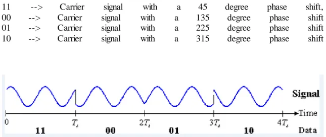
In QPSK the property that is changed is the phase, every two bits of a digital message which is transmitted is encoded in the carrier wave by changing its phase.

Any digital signal when taken as a pair of bits will have one the combinat io n 00,01,10,11.

The phase to symbol mapping could be different, meaning one could transmit carrier with 45-degree phase shift for 00. As long as the phase between consecutive of the 4 symbols differ by 90. QPSK will modulate as followed and represented in Figure 12.

24

11 --> Carrier signal with a 45 degree phase shift, 00 --> Carrier signal with a 135 degree phase shift 01 --> Carrier signal with a 225 degree phase shift 10 --> Carrier signal with a 315 degree phase shift

25 4. MIMO Systems

4.1.Introduction

Wireless propagation channels have been studied for several decades and are analyzed by hundreds of specialists. Thanks to that the results are a large number of channels models. The growing search for greater capacity in the wireless systems was the catalyst that resulted in various transmission techniques, including MIMO and Massive MIMO technology.

“In communications, MIMO is a technique that makes possible increase the capacity and reliability of a radio link using multiple transmit and receive antennas to exploit the spread of multiple paths. MIMO beginnings start at a 1970s research work on multicha nne l digital transmission systems and crosstalk between pairs of wires in a cable package”( A.R. Kaye and D.A. George, 1970).

Nowadays, it has become an essential element of wireless communication standards, including IEEE 802.11n (Wi-Fi), IEEE 802.11ac (Wi-Fi), HSPA + (3G), WiMAX (4G) and Long-Term Evolution (4G LTE).

MIMO technologies overcome the shortcomings of traditional methods through the use of spatial diversity. Data can be transmitted through N transmit antennas to N receive antennas supported by the receiving terminal. Such systems are used in wireless communication to improve capacity and bit error rate (BER). BER can be improved thanks to the spatial diversity obtained thought the large number of received antennas[9].

Significant increase is offered in data throughput and bandwidth without additiona l bandwidth or transmission power. These features are essential for the next generation of telecommunication systems.

Rayleigh fading was considered as the propagation channel for verification. Diversit y gain and spatial multiplexing (SM) are the two main advantages of MIMO systems that are used to study the effect of bit rate increase with increasing number of transmitting and receiving antennas. In the MIMO system, we mainly need to take spatial correlation into account. The spatial correlation effect should be minimized to obtain much better system performance.

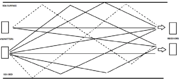
26 4.2.MIMO

In communications, MIMO makes possible increase the capacity and reliability of a radio link using multiple transmit and receive antennas to exploit the spread of multiple paths. The "MIMO" term, referred the mainly theoretical use of multiple antennas in both the transmitter and the receiver. In modern usage, "MIMO" refers specifically to a practical technique for sending and receiving multiple data signals on the same radio channel, at the same time via multiple-path propagation. In Figure 13, we can see what is a channel configuration of 2 transmit antennas and 2 receive antennas in a MIMO scheme. The MIMO is different from the intelligent antenna techniques developed to improve the performance of a single data signal, such as beamforming and diversity [10]. The MIMO technique applied in cellular systems brings four big improvements:

- increased data rate: due to use of more antennas, more independent data streams can be transmitted and more terminals can be attained simultaneously;

- improved reliability: increasing the number of transmit antennas creates more distinct paths for the radio signal to propagate, this is a good idea in the transmission because there are more rays of signal that will reach the receptor, and also good at the receiver because there are more rays that will reach the antennas and thus creating diversificat io n;

-Enhanced energy efficiency: the base station can concentrate its emitted energy rays in the spatial directions, where it knows that the terminals are localized;

-Low interference: The base station may intentionally avoid transmitting to directions where scattered interference would be harmful;

MIMO wireless technology is maturing and incorporated into recent and evolving wireless broadband standards. The more antennas the base station (or terminals) are equipped with, and the more degrees of freedom the propagation channel can provide, the better the performance in all four aspects above. However, the number of antennas used today is modest. The most modern standard, the LTE-Advanced, allows up to 8 antenna ports in the base station and the handsets being built today have far fewer antennas than that []. The gains in multiuser systems (MU-MIMO) are even more impressive because

27

such systems offer the ability to simultaneously transmit multiple users and the flexibi lit y of selecting which users are scheduled to be received at any time[11]

Figure 13 - A typical T=2 and R=2 MIMO system

But there are also disadvantages in the MIMO system, such as the greater complexity of the analog and digital domains. For point-to-point links, the complexity in the receiver is usually a greater concern than that of the transmitter. For example, the complexity of optimal signal detection increases exponentially with the number of transmit t ing antennas. In multiuser systems, transmitter complexity is also a concern, since advanced coding schemes must be used frequently to simultaneously transmit information to more than one user, while maintaining a low level of interference between users. This prohibitive complexity motivates a continuous search for computational efficie nc y, considering optimal or sub-optimal detectors.

4.3.Massive MIMO

The Massive MIMO is an emerging technology that increases MIMO by several orders of magnitude compared to the current MIMO system. With massive MIMO, systems can now use antenna arrays with a few hundred antennas, simultaneously serving many dozens of mobile terminals in the same time frequency resource. For example, a base station (BS) equipped with an array of active antenna elements M, using it to

28

communicate with single antenna terminals K. The basic premise behind the massive MIMO is mimic all the benefits of conventional MIMO, but on a much larger scale. The general multiuser MIMO concept has been around for decades, but the vision of actually deploying BSs with more than a handful of service antennas is relatively new [].

By making coherent processing of the signals through the array, a transmission precoding can be used in the downlink to focus each signal at its desired terminal, and the receive combination can be used in the uplink to discriminate the signals sent from differe nt terminals. In the downlink, this scheme would result in a set of directive bundles, as shown in Figure 14. Overall, Massive MIMO is a facilitator for the development of future (fixed and mobile) broadband networks that will be energy efficient, secure and robust and will use the spectrum efficiently. Each antenna unit would be small and active, preferably powered by an optical or electrical digital bus.

Figure 14 - Massive MIMO using beamforming credits to 5g.co.uk

Massive MIMO depends on spatial multiplexing that depends on the knowledge of the base station channel knowledge, both on the uplink and downlink. In uplink, this task can be easy to accomplish with the terminals sending pilots. Then, by combining these pilots and additional information that can be obtained from the data, the base station estimates the channel responses for each of the terminals. The downlink case turns out to be more difficult.

In conventional MIMO systems, such as the LTE standard, the base station sends pilot waveforms, on the basis of which the mobile terminals estimate the channel responses and quantify the estimates obtained and then feed them back to the base station. This will not be feasible on massive MIMO systems, at least not when operating in a high mobilit y environment, for two reasons:

29

• First, the ideal downlink pilots must be mutually orthogonal between the antennas. This means that the amount of time frequency resources needed by downlink pilots is sized as the number of antennas, so a massive MIMO system would require up to 100 times more resources than a conventional system;

Figure 15 - Passible massive MIMO antenna configuration, credits 5g.co.uk

• Second, the number of channel responses that each terminal must estimate is also proportional to the number of base station antennas. Thus, the uplink capabilit ie s needed to inform the base station about channel responses would be up to one hundred times greater than in conventional systems. Generally, the solution is to operate in Time division Duplex (TDD) mode and rely on reciprocity between uplink and downlink channels [14].

The massive canonical MIMO system operates in TDD mode, where uplink and downlink transmissions occur in the same frequency resource, but are separated in time. The physical propagation channels are reciprocal - which means that the channel responses are the same in both directions - that can be used in the TDD operation. In particular, massive MIMO systems exploit reciprocity to estimate uplink channel responses and then use the acquired channel state information (CSI) for the combination of uplink reception and downlink transmission pre-coding of payload data. Because transceiver hardware is

30

generally not reciprocal, calibration is necessary to explore channel reciprocity in practice. Fortunately, uplink and downlink hardware incompatibilities change only a few degrees over a one-hour period and can be mitigated by simple relative calibratio n methods, even without extra reference transceivers and relying only on mutual coupling between antennas in the array [16].

There are several good reasons to operate in TDD mode. Firstly, only the BS needs to know the channels to process the antenna signals coherently. Second, the overhead of the uplink estimation is proportional to the number of terminals, but independent of M. This makes the protocol fully scalable in relation to the number of service antennas. In addition, the basic estimation theory tells us that the quality of the estimation (per antenna) is not reduced by the addition of more antennas in the BS. In fact, the quality of the estimation improves with M if there is a known correlation structure between the channel responses on the matrix [3]. As the fading causes the channel responses to vary over time and frequency, the estimate and the payload transmission must fit into a time / frequency block in which the channels are approximately static.

The dimensions of this block are given by the coherence bandwidth Bc Hz and the coherence time Tc s, which conform to the transmission symbols τ = BcTc. Massive MIMO can be implemented using either single carrier or multiple carrier modulation.

Figure 16 - Possible Massive MIMO used in underwater ambient using acoustic transmission

31 4.4.MIMO Systems benefices

Due to the structure of multiple antennas and the possibility of jointly manipulating data at the ends of the communications link, the use of MIMO systems provides two types of gains in wireless communications systems, which are diversity gain and multiple xing gain. The diversity gain derives from the use of the multiple paths between the transmitting and receiving antennas of the system that suffer independent fading, for the transmission of signals that carry the same information, introducing robustness to the fading. Already the spatial multiplexing gain can be exploited by the parallel transmiss io n of different signals through the communications channel, which can be appropriately separated in the reception by the use of detectors, as uncorrelated decoder and has the objective of increasing the data transmission rate of the system. Usually these gains are antagonistic, that is, systems that maximize gains of diversity do not gain from spatial multiplexing and vice versa, but there is a possibility of establishing a balance between these two gains. In this section we will look at these gains in more detail.

4.4.1. Diversity Techniques

Classification of diversity techniques can be made by combining methods. In an effort to get the diversity gain, the signals from various channels need to be combined, and the combining method choosed affect the performance of the diversity technique used. The diversity combining methods increases the overall received power and that make a higher value of the SNR These methods are used to combine several replications of the transmitted signal, which undergo independent fading.[13] The 5 diversity techniques used and simulated in this paper are discussed below.

MFB – Matched filter bound is a model in which the Doppler normalized rate is unlimited, unrestricted. In contrast to the static channel case, the optimal matched filter receive is shown to be time varying and the probability of error is shown to depend on the transmission pulse shape. Matched filters are obtained by correlating a known signal, or template, with an unknown signal to identify the presence of the template in the unknown signal. This is the same as convolving the unknown signal with a conjugated time-reversed version of the template. The matched filter is the optimal linear filter for maximizing the signal to noise ratio (SNR) in the presence of additive stochastic noise.[14]

32

ZF - By employing spatial multiplexing, multiple- input multiple-output (MIMO) wireless antenna systems provide increases in capacity without the need for additional spectrum or power. Zero-forcing (ZF) detection is a simple and effective technique for retrieving multiple transmitted data streams at the receiver. If the transmitter knows the downlink channel state information (CSI) perfectly, ZF-precoding can achieve almost the system capacity when the number of users is large. On the other hand, with limited channel state information at the transmitter (CSIT) the performance of ZF-precoding decreases depending on the accuracy of CSIT. ZF-precoding requires the significant feedback overhead with respect to signal-to-noise-ratio (SNR) so as to achieve the full multiple xing gain[15]

MRC – Maximum ratio combining . the main ideia behind the MRC is the use of a linear coherent combining of branch signals so that the output SNR is maximized. In maximum ratio combining, all the branches are used at the same time. Each of the branch signals is weighted with a gain factor which is proportional to its own SNR. The co-phasing and summing is done for adding up the weighted branch signals in phase.

EGC - In Equal gain combining (EGC), the outputs of different diversity branches are first co-phased and weighted equally before being summed. (contrary to the MRC) After that the resultant output signal is connected to the demodulator. The weights are all set to one with the requirement that the channel gains are approximately flat and so constant and this is usually achieved by using an automatic gain controller (AGC) in the system.

IB DEF - it is known that nonlinear equalizers perform better than linear equalizers. iterative block decision feedback equalizer (IB-DFE) is na iterative FDE technique for SC-FDE that extended to diversity scenarios and layered space-time schemes. IB-DFE receivers can be regarded as iterative DFE receivers with the feedforward and the feedback operations implemented in the frequency domain. Because the feedback loop considers not just the hard decisions for each block, but also the overall block reliabilit y, the result is a small error propagation. Consequently, the IB-DFE techniques offer much better performances than the noniterative methods, with performances that can be close to the matched filter bound (MFB) and have low complexity equalization schemes since the feedback loop uses the equalizer outputs instead of the channel decoder outputs.[16]

33 4.4.2. Gain diversity

Traditionally, schemes with multiple antennas have been used to increase the diversity of the system in order to mitigate the fading existing in the communication channel and with that, to improve its reliability. Each pair of transmitting and receiving antennas provides a different route for the signals sent from the transmitter to the receiver of the system. By sending signals that carry the same information through each of these paths, replicas are obtained in the receiving antennas of the system after suffering independent fading in the communication channel, so that, if we process them properly in the receiver, a more reliable detection of the signals will be possible transmitted.

The gain of transmission diversity can be obtained when we have the same signal being transmitted through multiple transmitting antennas of the system, generating differe nt replicas of this signal at the reception, as shown in Figure 17 . Each of these replicas, when transmitted by the communications channel, has undergone a different fading along the channel path, and the receiver must handle these signals to obtain the estimate of the transmitted signal. In systems with gain of diversity of reception, Figure 18 we have that the signal sent by the transmitting antenna is received by multiple receiving antennas, in each one of them we will have a sample of the signal transmitted differently faded. For error to occur in reception, all paths must undergo deep fading simultaneously. However, this event occurs with small probability.

The diversity gain provides the system with an increase in the signal-to-noise ratio or a reduction in the transmission power required to obtain a given error rate. He can be defined as the slope of the error probability curve in Logarithm log scale given by:

𝑑 = − lim 𝜌→∞

log(𝑃_𝑒(𝜌)) log(𝜌)

Where 𝑃𝑒 is the mean error probability and 𝜌 is the signal-to-noise ratio in each of the receiving antennas of the system. In a system with 𝑁_𝑇 transmitting antennas and 𝑁_𝑅 receiving antennas.

34

Figure 17 - Gain diversity in transmission

Figure 18 Gain diversity in reception

Whose channel has dimension 𝑁_𝑅 × 𝑁_𝑇, the diversity gain has maximum heat given by the channel dimension, that is, by 𝑑_𝑚𝑎𝑥 =𝑁_𝑅× 𝑁_𝑇, which is the total number of possible independent paths in the communications link.

Another interpretation for the diversity gain is that this value measures how much the MIMO transmitter can exploit the channel's multiple paths to provide robustness to fading, making the system more robust, exploiting the diversity gain decreases the probability of error of the channel. (Pe), since the probability that all the signal- o nly replicates undergo deep fading becomes much reduced, and this logically improves the reliability of the system and the quality of service it offers. Since the fades between the independent antenna pairs and the diversity gain obtained in the given system by d, the error probability for these systems decays in the form of (𝑝 −𝑑 (raised to minus 𝑑). For high values of 𝑝. In contrast we have that the probability of error of a system with only one transmitting antenna and one receiving antenna decays in the high 𝜌 firm at least one.

35 4.4.3. Spatial multiplexing gain

In addition to gaining diversity, another way of exploiting the fading of the wireless communications channel using MIMO system is to benefit from the degrees of freedom available in this communications system due to its multiple transmitting and receiving antennas in order to increase the data transmission. The degrees of freedom of a system can be defined as the spatial dimension of the received signal, i.e. the number of differe nt signals that can be clearly distinguished at the receiver. As we shall see, this characterist ic can be verified when analyzing the capacity measures of the communications channel In an ergodic channel whose statistical properties such as its mean and variance can be deduced from a single sample sufficiently long to perform this channel or from a single sample of many embodiments whose communications system has 𝑁_𝑇 transmit t ing antennas, 𝑁𝑅 antennas and path gains between each pair of Rayleigh fading antennas, represented by the channel H matrix elements and modeled as independent and identica lly distributed random variables, the ergodic capacity is given by:

𝐶(𝜌) = E {log [𝑑𝑒𝑡 (I𝑁_𝑅 + 𝜌

𝑁_𝑇𝐻𝐻′)]}

Where E{} is the operator of hope and p is the signal-to-noise ratio at each receiving antenna of the system. Considering high values of P and the elements of the matrix of the independent communications channel, we can write this formula as in:

𝐶(𝜌) ≈ 𝑚𝑖𝑛{𝑁𝑇, 𝑁𝑅} log ( 𝜌 𝑁_𝑇) + ∑ E 𝑚𝑎𝑥{𝑁_{𝑇 ,}𝑁_𝑅} 𝑖= |𝑁_𝑇−𝑁_𝑅|+1 {log 𝑋_2𝑖2_}

Where 𝑋_2𝑖2 is a chi-square variable with 2𝑖 degrees of freedom. We observed that for high values of p the channel capacity grows in the proportion of the 𝑚𝑖𝑛{𝑁_𝑇, 𝑁_𝑅} × log(𝜌), in contrast to log(𝜌) for can is with only one antenna at each end of the link. This result suggests that the channel of multiple antennas can be seen as N =𝑚𝑖𝑛{𝑁_𝑇, 𝑁_𝑅} non - interfering parallel channels, where N is the total number of degrees of freedom of the system. In the case of the path gains of the communication channel between the transmitting and receiving antennas of the system m data per ℎ_𝑖𝑗, have independent fading, the antennas are sufficiently spaced from each other so that the signals are able to