Influence of the electrotonic architecture on single neurons dynamics : a computational approach

(1)

Faculdade de Ciências| Faculdade de Letras| Faculdade de Medicina| Faculdade de Psicologia

Influence of the Electrotonic Architecture on Single

Neurons Dynamics: a Computational Approach

André Castro

DISSERTAÇÃO DE MESTRADO

UNIVERSIDADE DE LISBOA MESTRADO EM CIÊNCIA COGNITIVA

(2)

(3)

Faculdade de Ciências| Faculdade de Letras| Faculdade de Medicina| Faculdade de Psicologia

Influence of the Electrotonic Architecture on Single

Neurons Dynamics: a Computational Approach

Autor:

André Castro

Projeto orientado por: Prof. Luís Correia

DISSERTAÇÃO DE MESTRADO

UNIVERSIDADE DE LISBOA MESTRADO EM CIÊNCIA COGNITIVA

(4)

(5)

To my Mother:

She is a kind hearted woman in a hateful world who caught every thing that life ever hurled, but like the oldest mountain she always stood so tall, forever showing what it means to be unbreakable. She was the one who taught the sun

(6)

(7)

Acknowledgements

First and foremost, I would like to thank my supervisor Professor Luís Correia for all his guidance and patience. Professor Luís gave me the chance to freely explore through a number of research options, without ever feeling anything but utmost support from him.

Second, I would like to thank Dr. Rob Mills who gave up his time to provide several contributions and insights into many aspects of this thesis. I owe Dr. Mills my gratitude for that.

A special thanks to all my fellows from the Cognitive Science Program. Partic-ular acknowledgements to Marco Nunes, Bruno Penha and Rafael Nascimento for providing me with stimulant discussions and companionship.

To my childhood friends, for showing me that besides a world to understand there is a life to live.

Last but not least, I have to thank my family, without their unconditional and unwavering support I would have never achieved my goals in life. I owe my future success and happiness to you all, you mean everything to me. To my Mother, Father, Grandmother Maria, Grandfather Zé and sweet Pipinhas, the biggest thank you of all. I will always love you.

(8)

(9)

Resumo

Na presente dissertação, investigamos de forma sistemática a forma como a morfologia dendrítica subjaz as diferenças na atividade elétrica neuronal que estão na base da geração de potenciais de ação. De forma a atingir este objetivo desenvolvemos uma medida que quantifica as duas maiores fontes de variabilidade morfológica: métrica e topologia, e ainda outros componentes estruturais como canais iónicos. Baseado na nova medida, propomos um novo mecanismo de sincronização que relaciona a estrutura dendritica à modulação de currente axial que flui da árvore dendrítica até ao soma. Esta hipótese afirma que quanto mais simétrica a estrutura electrotónica da célula é, mais currente irá chegar ao soma das dendrites devido à sincronização obtida em virtude da simetria estrutural.

De forma a testar a hipótese de sincronização foram simuladas duas exper-iências usando modelos multi-compartimentais computacionais de células de Purkinje, Piramidais e células do córtex Visual. Na primeira abordagem, as estruturas das células foram quantificadas utilizando a nova medida e depois comparadas com a quantidade de currente axial proviniente das dendrites que atingia o soma. Na segunda abordagem, os potenciais de voltagem são medidos ao nível do compartimento axo-somático de forma a se poder analisar se difer-enças encontradas na condição axial induzem diferdifer-enças na atividade de spiking da célula. Os resultados apoiam a hipótese de sincronização, pois neurónios com estruturas electrotónicas com níveis de simetria mais elevados, exibem os níveis mais elevados de currente axial a chegar ao soma para o mesmo estímulo. As diferenças encontradas na condição axial correlacionaram-se com o tempo que os neurónios levaram a atingir um potencial de ação, com os neurónios mais simétricos a requerer menos tempo para o fazer. No entanto, diferenças significativas não emergiram nos padrões de potenciais de ação, mas estes resul-tados podem ser explicados por algumas limitações no protocolo de estimulação. Em suma, os nossos resultados mostram que a medida desenvolvida é uma alternativa promissora às abordagens morfométricas tradicionais, pois pode ser utilizada com confiança para quantificar diferenças estruturais, podendo ser aplicada a vários tipos de neurónios, providenciando uma ligação entre estrutura e função.

Palavras-chaves: Estrutura-Função, Simetria, Estrutura Electrotónica, Sincronização

(10)

(11)

Abstract

In this dissertation, we systematically investigate how dendritic morphology underlies the differences in the electrical dynamics of the cell that lead to spiking behaviour. To accomplish this goal we develop a new measure that provides a quantitative account of the two most relevant sources of morphological variability: metrics and topology, as well as of other structural components such as ion channels. Supported by the new measure, we propose a new synchronization mechanism that relates dendritic structure to the modulation of axial current that flows from the dendrites to the soma. This hypothesis states that the more symmetric the electrotonic structure of a cell is, the more current will reach the soma from the dendrites due to the synchronism obtained by virtue of structural symmetry.

To test the synchronization hypothesis two simulation-based experiments using detailed multi-compartmental computational models of Purkinje, Pyrami-dal and Visual cortical cells were conducted. In the first approach, by means of the novel measure, the structure of the cells are quantified, and compared with the amount of axial current reaching the soma from the dendritic tree. In the second approach, voltage traces are measured at the axo-somatic com-partment to analyse whether differences found in the axial current condition induce differences in the output spiking patterns. Our results support the synchronization hypothesis, as neurons with electrotonic structures with higher levels of symmetry exhibited the highest amount of current reaching the soma for the same stimulus. These differences correlated with the time that neurons required to spike, with more symmetrical neurons requiring less time to do so. Nevertheless, significant differences fail to emerge in the output spike trains, but these results can be explained by some limitations in the stimulation protocol. Overall, the results show that the proposed measure is a promising alternative to traditional morphometrics measures as it can be used with confidence to quantify structural differences, and can be applied across different types of neurons while providing a bridge between structure and function.

Keywords: Shape-Function, Symmetry, Electrotonic Structure, Syn-chronization

(12)

(13)

List of Figures

2.1 The different levels of analysis in Neuroscience and their specific types of

computational models. . . 8

2.2 Steps involved in the construction of a computational model . . . 9

2.3 Neuron cell diagram . . . 10

2.4 EPSP attenuation due to passive dendrites properties . . . 11

2.5 Brainstem auditory neuron coincidence detection algorithm . . . 12

2.6 Action potential mechanism . . . 13

2.7 Compartmentalization of a neuron . . . 18

3.1 Diversity of dendrite morphologies . . . 22

3.2 Metrical and topological morphometrics terminology . . . 25

4.1 Perovskite crystal structure . . . 32

4.2 Example of dendritic branch translated into a graph . . . 33

4.3 Vertex automorphisms of the star graph S4 . . . 35

4.4 Symmetry ratio visualization . . . 38

4.5 Size effect visualization . . . 38

4.6 Electrotonic path illustration . . . 39

4.7 e−X _{and X factor relation. . . .} ₄₀

5.1 Shape diagram of the original collected neurons. . . 44

5.2 Work flow from the cells artificial reconstructions . . . 45

5.3 Fitting plots for the e−X vs. axial current relation . . . 50

5.4 Fitting plots for the e−X vs. time to spike relation . . . 53

5.5 Average spiking rate plot for the three cell types . . . 54

A.1 All the different trees with eight nodes . . . 60

(16)

(17)

List of Tables

2.1 Basic computations that follow from generic neuronal properties . . . 13

3.1 List of topological morphometric measures . . . 24

3.2 List of metrical morphometric measures . . . 25

5.1 Morphometric statistics of the original collected trees after processing. . . 44

5.2 Simulations Parameters . . . 47

5.3 Fitting parameter values and residues analysis for the e−X vs. axial current . . 49

5.4 Fitting parameter values and residues analysis for the e−X vs. time to spike. . 54

A.1 Measures comparison results . . . 60

(18)

(19)

List of Symbols

Symbol Units Description

d µm Diameter of the neurite

l µm Length of the compartment

Rm Ωcm2 Specific membrane resistance

Rin Ωcm2 Specific input resistance

Cm µFcm−2 Specific membrane capacitance

Ra Ωcm Specific axial resistance

rm Ωcm Membrane resistance per inverse unit length

cm µFcm−1 Membrane capacitance per unit length

ra Ω/cm−1 Axial resistance per unit length

V mV Membrane Potencial

Em mV Leakage reversal potential due to different ions

I µAcm−2 Membrane current density

Ie nA Injected current density

Ic nA Capacitive current

Ii nA Ionic current

f Hz Frequency

∆t µs Time-step of the numerical integration nseg Number of compartments of a given neurite

Na+ _{Sodium ion}

Ca++ _{Calcium ion}

K+ _{Potassium ion}

dλ dλ rule

τm msec Membrane time constant

λ µm Space constant

¯

gleak pS µm−2 Membrane maximum leakage density

¯

gN a pS µm−2 Fast sodium maximum conductance density

¯

gKm pS µm−2 Slow voltage-dependent non-inactivating

potas-sium current maximum conductance density

(20)

xvi LIST OF SYMBOLS

¯

gKv pS µm−2 Fast non-inactivating potassium current

maxi-mum conductance density ¯

gKca pS µm−2 Slow calcium- activated potassium current

maxi-mum conductance density ¯

gCa pS µm−2 High voltage-activated calcium current maximum

conductance density

dsyn pS µm−2 Synaptic maximum conductance density

(21)

Chapter

1

Introduction

In this first chapter, we start by putting the present work into a bigger perspective and enumerate the main objectives of the research presented in the following manuscript. In the final section of the chapter, we provide an overview of the thesis structure.

1.1 Context

The shape–function paradigm, i.e., the existence of a close link between shape and function in nature, probably takes origin along with the beginning of human scientific thinking. This paradigm finds an excellent field of application in Neuroscience in a branch named Neuromorphology. This field yields not only the application of a set of techniques useful to measure and characterize the geometrical properties of nerve cells and structures, but more extensively cares about studying the relationship between the geometry of the nervous structure and its functionality [8]. In particular, this thesis is on the subject of how the structural features of single neurons may influences the electrical activity of the cell and its firing behaviour .

However, the task of relating structure to function is not an easy one because the brain is a extraordinarily complicated circuit. To make things more complicated the components of this circuit are not homogeneous, but instead, there are many different classes of neurons [15]. To fully understand the function of any circuit both the components and the connections must be identified and understood, but this is an extremely difficult task when considering the number of neurons in the brain [60].

Nevertheless, experimental and theoretical observations disclose many structural and functional patterns, leading one to think that must be underlying organizational principles that govern brain structure and allow the network to function [24].

Fundamental Research

One of the central questions in neuroscience is how particular tasks, or computations, are implemented by neural networks to generate behaviour. The prevailing view has been that information processing in neural networks results primarily from the properties of

(22)

2 CHAPTER 1. INTRODUCTION

synapses and the connectivity of neurons within the network, with the intrinsic excitability of single neurons playing a lesser role [69]. As a consequence, the contribution of single neurons to computation in the brain has long been underestimated .

However, in recent years, the role of neurons in these computations has evolved conceptually from that of a simple integrator of synaptic inputs until a threshold is reached and an output pulse is initiated [73], to a much more sophisticated processor with mixed analog-digital logic and highly adaptive synaptic elements [37, 59].

During this conceptual transition, it was realised that the morphology of a neuron, notably its dendrites, play a critical role in brain function for two main reasons [59]. First, neuronal morphology defines and is defined by the circuitry, being the synaptic contact between the output axon of one neuron and the input dendrite of another the major element of neuronal connectivity. As such, a precise morphology is crucial to establish the connectivity required for the nervous system to operate normally. Secondly, the precise morphology of a neuron and its membrane’s ion channel composition set the computations that a neuron performs on its inputs, i.e., the propagation and integration of synaptic input signals along the neuron’s membrane up to the axon initial segment, the location where the neuronal output is typically generated. Therefore, it has been hypothesised and demonstrated in some cases that neurons with different structures serve different functions or endow different computational capabilities [24].

In spite of it is nowadays a given fact the existence of a link between structure and function, the mechanisms underlying this link are poorly understood, and consequently the impact of morphological differences on the cell behaviour remains insufficiently known [69, 88]. This situation is a consequence of the complexity of single neurons: these cells have many branches with irregularly varying diameters and lengths, their membranes are populated with a wide assortment of ionic channels that have different ionic specificities, and kinetics dependent on voltage and second messengers. Trying to incorporate every of these biological details may obscure the focus on the essential structure-function relation, whereas limiting investigations to highly abstract processes may reduce the biological relevance of specific findings.

Moreover, scattered over the surface of the cell may be hundreds or thousands of synapses, and synapses themselves are far from simple, often displaying stochastic and use-dependent phenomena that can be quite prominent, and frequently being subject to various pre and postsynaptic modulatory effects. In sum, even a single isolated neuron is an intricate world on its own [49].

Despite this daunting complexity, even if the brain was perfectly static, it seems unlikely that the genome could encode the location of every synapse and therefore the location of every piece of a dendritic tree and axon from every neuron. It seems probable that the genome specifies general rules, mechanisms or strategies for connectivity and structure, and then connections form within the context of these general rules [8]. The long-term end result of the collective effort by researchers in Computational Neuroscience at large is

(23)

1.2. RESEARCH OBJECTIVES 3

to identify these general rules and build a comprehensive structural and functional model of the brain [72]. Such a model might have deep implications for scientific understanding as well as technological development.

Translational Research

The unravelling of these general rules not only has importance for fundamental purposes but also has many possible important applications at different levels. For example, various studies report that many neuropsychiatric disorders are characterized by dendritic and synaptic pathology, including abnormal spine density and morphology, synapse loss, and aberrant synaptic signaling and plasticity [57, 66, 93]. Therefore, identifying and understanding these changes in neuronal morphology are essential for understanding brain function in normal and disease states.

Moreover, theories and methods of bio-inspired Artificial Intelligence, such as Neural Engineering, aim at reproducing the functionalities of brains in order to engineer intelligent machines. Issues addressed by Neural Engineering that Computational Neuroscience may help shed a light on include high-level architectures that could reproduce cognitive abilities, brain-computer interfaces and implementation of neural models in hardware [34, 46, 50].

1.2 Research Objectives

Taking into account what was previously mentioned, the scientific issue that motivates the design and construction of the models analysed in the present thesis, is the question of how signal integration is affected by the structure and biophysical properties of neurons. Especially, the objectives of the present manuscript are:

• Systematically investigate how the physical parameters controlled by dendritic mor-phology underlies the differences in the electrical dynamics of the cell that leads to spiking behaviour.

• The developed approach should provide a quantitative account of the two sources of morphological variability: metrics (size of the dendritic tree, segment lengths, segment diameters) and topology (the way the segments of the dendritic tree are connected) and possibly of others structural components such as ion channels. • Since there are not any such measures in the literature, one of the main goals of the

research conducted was to create a measure as general as possible, i.e., that could be applied across many types of neurons.

1.3 Research Contributions

(24)

4 CHAPTER 1. INTRODUCTION

• This thesis is the first to introduce in the Computational Neuroscience domain a measure, e−X_{, that quantifies topological, metrical, passive and active properties of}

neurons in a unified way.

• Our results show that e−X _{has a highly discriminative power, and it provides a direct}

bridge between structure and function. We compare e−X to other more traditional approaches.

• Based on the novel measure it is proposed a new structure based mechanism that neurons may explore to integrate electrical signals. We hypothesised how symmetric electrotonic dendritic structures lead to better electrical signals synchronization. • Using computational models of artificial reconstructed neurons, we manipulate the

dendritic mechanism to determine if there is a causal link between the proposed mechanism and the electrical behaviour of the cells. Our simulation-based experiments show that the proposed mechanism is a robust and important factor modulating axial current that causes neurons to spike.

1.4 Report Overview

In this section, we provide an overview of the thesis structure. In Chapter 2, we review the state-of-the-art on the distinct subjects relevant to this dissertation. The chapter is divided into three main sections that are dedicated respectively to the computational approach in Neuroscience, the role of single neurons in information processing, and to the realistic modelling of single neurons.

In chapter 3, we discuss the morphological features of dendritic tree structures, providing an overview of quantitative procedures used to accomplish that. The main focus of the chapter is on the description of morphological complexity of neurons and how one can use this description to unravel neuronal function in dendritic trees and possibly in neural circuits.

In chapter 4, we describe and discuss some advanced preliminaries, necessary in order to understand the theoretical part of the research presented. Basically, we derive and introduce a new measure that relates structure to function in single neurons, and in the end of the chapter the research problem is stated.

In chapter 5, it is provided a description of the approach and method employed to solve the stated problem, and in the final section of the chapter the results found are analysed and discussed.

In chapter 6, the work done in the present thesis is positioned in the context of other people’s efforts in the area. It is shown the principal differences and similarities with respect to the details of the problem, the approach, the results, and the methodology. Then we discuss directions for future work. Finally, we give a summary of the report and present some conclusions.

(25)

Chapter

2

Background

This chapter includes a broad range of subjects relevant to this dissertation. The subjects are presented in a top-down fashion. First, we are going to expose the reader to the field of Computational Neuroscience, particularly to its advantages and disadvantages, and how Neuroscience as a whole can benefit from this approach. Afterwards, we are going to review the state of the art of single neuron computational abilities, this means how they process information in order to execute certain tasks, providing theoretical and experimental examples to support. In the final section of the present chapter, we will introduce the techniques used to implement morphologically realistic models of single neurons.

2.1 The Computational Approach

The use of computational tools to Neuroscience is known by a number of largely synonymous names, such as Computational Neuroscience, Theoretical Neuroscience or Computational Neurobiology. This field has a twofold approach: in one hand, it comprehends the use of databases, the World Wide Web, visualization of data, storage and analysis of Neuroscience data [6, 22, 78]. On the other hand, it attempts to analyse computational models of the nervous system by using powerful computers to find numerical solutions to the complex sets of equations needed to construct an appropriate model of certain parts of the nervous system [16, 20, 38].

2.1.1 What is a Computational Model?

The complexity of the nervous system makes it very difficult to someone to theorise about it, in a convincing manner, on how such system is put together and how it functions. To aid our thought processes we can represent our theory as a computational model in the form of a set of mathematical equations. The variables of the equations represent specific neurobiological quantities, such as the rate at which impulses are propagated along an axon, or the frequency of opening of a specific type of ion channel, and the equations

(26)

6 CHAPTER 2. BACKGROUND

themselves represent how these quantities interact according to the theory being expressed in the model [16, 20, 37, 41].

Advantages

A key advantage of computer modelling is its ability to wrestle with complexity that often proves daunting to otherwise unaided human understanding, and because of this, the use of computer models to understand how the brain works has been a critical contributor to scientific progress in this area over the past few years. Solving these equations by analytical or simulation techniques enables us to show the behaviour of the model under given circumstances, and thus address the questions that a certain theory was designed to answer [16, 20]. By doing so, these models can be used as explanatory or predictive tools, removing ambiguity from theories and complement empirical experiments (sometimes some computational models can even explore conditions that are very difficult to test empirically).

Disadvantages

Nevertheless, in all fields where computer models are used, there is a fundamental distrust of these models. They are themselves complex, created by people, and have no necessary relationship to the real system in question.

A key aspect of computational modelling is determining values for model parameters and often these will be estimates at best, or even complete guesses. To avoid this drawback, a good model must be constrained by empirical data at as many levels as possible, and they must generate predictions that can then be tested empirically [41].

Another known issue in computational modelling in general, and in computational modelling applied to Neuroscience in particular, is the trade off between incorporating sufficient details to account for biological complexity, and reducing this complexity to a bare minimum to make the model tractable [49]. The nature of the scientific question that drives the modelling work will largely determine the level at which the model is to be constructed, and therefore the level of details to be incorporated, but the general rue of thumb is to develop the simplest possible model that captures the most possible data. Often this is a matter of judgement on what phenomena someone regards as being important, and once again, this will vary depending on the scientific questions being addressed with the model.

2.1.2 Developing a Computational Model

To develop a computational model in neuroscience the researcher has to decide how to construct and apply a model that will link the neurobiological reality with a more abstract formulation that is analytical or computationally tractable. As previously mentioned, guided by neurobiological data, decisions have to be made about the level at which the

(27)

2.2. THE SINGLE NEURON 7

model should be constructed, the nature and properties of the elements in the model and their number, and the ways in which these elements interact. Having done all this, the performance of the model has to be assessed in the context of the scientific question being addressed.

Conceptual Model

The first step is to formulate a conceptual model that attempts to capture just the essential features that underlie a particular function or property of the physical system. If the aim of modelling is to provide insight, then formulating the conceptual model necessarily involves simplification and abstraction [16, 20, 41].

When we formalize our description of a biological system, the first language we use is Mathematics, by doing so one specify the theory in a non-ambiguous and precise way. The conceptual model is usually expressed in mathematical form, although there are occasions when it is more convenient to express the concept in the form of a computer algorithm.

Section 2.2.3 is concerned with mathematical and conceptual representations of phe-nomena relevant to model single neurons.

Computational Model

A computational model is a working embodiment of a conceptual model through the medium of computer simulation [16, 20, 41]. It can assist hypothesis testing by serving as an artificial laboratory preparation in which the functional consequences of the hypothesis can be examined. The conceptual model, and the hypothesis behind it, determine what is included in the computational model and what is left out.

Such tests can be valid only if the computational model is as faithful to the conceptual model as possible. This means that the computational model must be implemented in a way that does not impose additional simplifications or introduce new properties that were not consciously chosen by the user. Otherwise the interpretation of the results obtained can become compromised, because they just might be a byproduct of distortions produced by trying to implement the model with a computer.

Section 2.3 of the present chapter will deal with the techniques used in the constructions of morphologically realistic models of single neurons.

2.2 The Single Neuron

The fundamental building block of every nervous system is the single neuron. Understand-ing how these sophisticated elements operate is an integral part of the quest to solve the mysteries of the brain. An important contemporary concept of the neuron doctrine is that the neuron is made of several regions with different functions interacting in complex ways

(28)

8 CHAPTER 2. BACKGROUND Nervous System 1 m Subsystems 10 cm Neural Networks 1cm Microcircuits 1mm Neurons 100 µm Dendritic subunits 10 µm Synapses 1 µm Signaling Pathways 1 nm Ion Channels 1 pm Neural Fields Networks of Sim-plified Neurons Cascade and Black-box Models Reduced Compart-mental Models Multi-compartmental Models

Figure 2.1: To fully comprehend the nervous system it is required to understand it at many different levels, at spatial scales ranging from metres to nanometres or smaller. At each of these levels there are different computational models for how the elements at that level function and interact. The appropriate level of description depends on the particular goal of the model.

Multi-compartmental Models: morphologically realistic models that focus on how the spatial

structure of a neuron contributes to its dynamics and function [49, 41]. Reduced

Compart-mental Models: these models offer a good compromise between realism and computational

efficiency when studying single neurons [49, 41]. Cascade and Black-Box Models: these models are the highest level models for single neuron modelling, and basically they are simplified functional models of neural spike responses [49]. Neural Networks of Simplified Neurons: interconnected sets of reduced compartmental neurons that simulate the function of biological neural networks, such as synchronization and oscillations [37]. Neural Fields: are even higher level models of neural networks; the equations are tissue level models that describe the activity (i.e. pattern formation) of large chunks of neurons populations [37].

(29)

Neuronal Component Conceptual Model Computational Model

Figure 2.2: Creating a computational model of neuronal component/phenomena involves two steps. The first step deliberately omits real-world complexities to produce a conceptual model. In the second step, this conceptual model must be faithfully translated into a computational

model [20].

and these functionally diverse regions correspond to anatomically distinct parts of the cell [56].

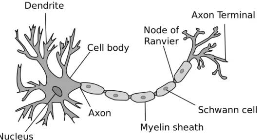
The axon is a component of a neuron specialized to distribute or conduct nerve impulses generally over great distances. It is smooth and only sends off branches at long intervals, if at all. It is commonly surrounded by a barrier of non-nervous cells called neuroglia inside the central nervous system, and schwann cells outside (see Figure 2.3).

The dendrites are tree-like structures specialized for collecting information from other neurons, neuroglia, circulating hormones and extracellular signals to the cell body or soma. Vertebrate dendrites are commonly highly branched, irregular in thickness, thorny and are covered by cocktail of excitable channel types. The neuronal cell membrane, explores its permeability to different ions and concentration gradients across the membrane to perform complex manipulations of signals representing internal and external worlds.

In the following subsections, we will provide an overview of Cable Theory applied to model the spread and propagation of voltage and currents in neurons. This approach started with Wilfrid Rall’s seminal contributions in the sixties [83]. Particularly, the equations that are going to be presented in the following pages constitute the base of the multi-compartmental models used later in this thesis.

2.2.1 Dendritic Integration

The input-output relation in neurons can be studied in two opposing points of views:

neural encoding and neural decoding [27]. On one hand, neural encoding refers to

the study of how neurons respond/integrates a particular stimulus, and the construction of models that attempt to predict the response to those stimuli. This is the topic of the present subsection.

In the other hand, neural decoding is concern with analysing the amount of information encoded by sequences of action potentials. This issue will be briefly exposed in the following subsection 2.2.2.

A typical neuron receives inputs from thousands of other neurons through the contacts on its synapses (see Figure 2.3), and dendrites receive the far majority of these synaptic inputs [56]. The inputs produce electrical transmembrane currents that change the membrane potential of the neuron. Synaptic currents produce changes, called postsynaptic

(30)

Figure 2.3: The axon terminal buttons are the connection points between sending neurons (pre-synaptic) and the synapses of receiving neurons (post-synaptic). Most synapses are on

dendrites, which is where the neuron integrates all the input signals. Then, all these signals

flow into the main dendritic trunk and into the cell body or soma, where the final integration of the signal takes place. The thresholding takes place at the start of the axon, named axon

hillock. The axon also branches widely and is what forms the other side of the synapses onto

other neuron’s dendrites, completing the next chain of communication [56].

potentials (PSPs). Small currents produce small PSPs; larger currents produce significant PSPs that can be amplified by the voltage-sensitive channels embedded in the neuronal membrane and lead to the generation of an action potential or spike – an abrupt and transient change of membrane voltage that propagates to other neurons via the axon [56].

In an active neuron the superposition of passive and active electrical properties serves to allow the cell the possibility of summing the transmembrane potential either linearly or nonlinearly and to reach depolarization levels sufficiently high to trigger action potentials [84].

Passive Properties

Even though it is rare to find fully passive dendrites in the mammalian brain, i.e., that do not contain voltage-dependent membrane conductance, it is important to recognize that the passive properties of the dendritic tree provide the backbone for the electrical signalling in dendrites, and enhance the computational power of neurons, making understanding the passive properties of dendritic trees crucial for the fully comprehension of the single neuron computations [60, 83].

In terms of signal propagation, dendrites behave like electrical cables with medium-quality insulation, and this propagation depends on Rm and Cm that may vary from cell

to cell [60, 84]. As such, passive dendrites linearly filter the input signal as it spreads to the soma, where it is compared with the threshold. This filtering tends to attenuate and temporally delay the dendritic signal as a function of the distance it travels and the frequency of the original signal. Thus a brief and sharp excitatory postsynaptic potential

(31)

Figure 2.4: Voltage traces of EPSP recorded ate the soma, from synapses located away from the soma and close to the soma. Passive dendrites function as a low-pass filter and slows the time course as measured at soma, thus increasing temporal summations at the soma.

(EPSP) that originates in the dendritic tree will be transformed into a much smaller and broader signal when it arrives at the soma. Nevertheless, these factors are not the only factors that influence the PSPs propagation in a dendritic tree. The geometry of the dendritic tree, coupled with a unique synaptic architecture, influences signal propagation as well and may implement specific computations [45, 84].

Synaptic events are conductance changes, rather than voltage sources, and their interaction is significantly constrained by dendritic morphology. Spatial summation describes the interaction of coincident synaptic inputs and depends on their relative locations within the dendritic tree, and temporal summation describes the interaction of coincident synaptic inputs and depends on their relative offset and time course (which itself depends on τm = Rm∗ Cm) [84]. One important result regarding these two types of

summation is that sublinear summation is expected for synapses located close together (or temporally correlated), but it is minimal, or non existent for spatially (temporal) separated inputs. However, this sublinear summation is modulated by interactions between spatial and temporal summation, with summation reaching almost linear additivity when a certain balanced is reached between the two. For example, if two synapses are contiguous spatially, the summation is maximum when a certain amount of temporal delay between the onset of both happens, and vice-versa, until a limit is reached and the two synapses do not interact electrically. This happens because the depolarization caused by one synaptic event reduces the driving force at nearby synaptic locations [45]. These principles governing dendritic integration of EPSPs apply similarly to IPSPs (inhibitory postsynatic potentials).

Taking into account the principles stated, and the interaction between excitatory and inhibitory PSPs, it is obvious that with certain synaptic arrangements in a passive dendritic tree alone, nonlinear computations can be implemented (see Figure 2.5 as an example).

Active Properties

Many types of neurons display voltage-dependent membrane conductances in their den-drites. The presence of these active conductances in dendrites has important consequences for synaptic events and their integration. Depending on their voltage dependence, ionic specificity, and kinetics, dendritically expressed voltage-gated channels have the

(32)

poten-12 CHAPTER 2. BACKGROUND

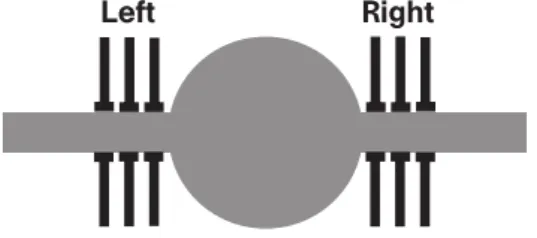
Figure 2.5: Neuron model that mimics the algorithm implemented by auditory neurons. The model consists of a soma (centre) and two cylindrical dendrites. The task of a brainstem auditory neuron is to perform coincidence detection in the sound localization system, i.e. it has only to respond if the inputs arriving from both ears coincide in a precise manner, while avoiding a response when the input comes from only one ear. Inputs to each ear do not produce strong enough PSPs, but the input from both ears is summed and compared with threshold, and this sum exceeds the threshold, whereas if the input arrives only to one ear the output is not large enough. Agmon-Snir et al. [1] showed that dendrites of these neurons might implement a similar algorithm. This is an example of how the dendritic tree geometry, coupled with a unique synaptic architecture, implements specific computations that are beneficial for single neurons computations. (This picture was taken from [1])

tial to amplify, dampen, and shape synaptic responses as they propagate through the dendritic tree, expanding the computational repertoire of a neuron [59, 60, 69]. While a comprehensive discussion of all dendritically expressed channels is beyond the scope of this review, several dendritic conductances stand out at being especially important for synaptic integration across a wide range of neurons, such as:

• active dendrites can influence the integration of PSPs is by amplification of inputs, because the fact that passive dendrites attenuate the synaptic input. There have been proposed several mechanisms, all off them with experimental support, for this, namely sypnatic scaling, subthreshold boosting, local dendritic spikes, global dendritc spikes [69, 21].

• interactions between voltage-dependent conductances can also underlie the generation of intrinsic subthreshold oscillations, which have been demonstrated in various cell types (e.g. place fields in hippocampus [3]).

• strong local dendritic nonlinearities, caused by the presence of voltage-gated and calcium channels, may transform a dendritic tree in a set of multiple subunits, such as single dendritic branches, that independently process input and convey the signal to the soma through an amplitude boosting nonlinearity [35, 69].

Besides the information just stated, there are many other ways in which voltage-dependent conductances can shape membrane-potential dynamics and neural computation that we have not reviewed here.

(33)

Computation Biophysical Mechanism

Addition or subtraction Dendritic summation of excitatory and/or inhibitory inputs

Subtration Shunting inhibition plus integrate-and-fire mechanism

Multiplication or division Synaptic interaction

Gain modulation via synaptic background noise

High-pass filter Firing rate adaption

Low-pass filter Passive membrane properties

Toggle switch Bistable spike generation

Table 2.1: Basic computations that follow from generic neuronal properties. These simple computations can be used together in the same neuron to create algorithms that process the information in a behavioural relevant way, e.g. collision avoidance, sound localization, motion detection [49].

Figure 2.6: Action potentials are generated and sustained by ionic currents through the cell

membrane. The ions most involved are sodium, Na+_{, and potassium, K}+_{. In the simplest case}

an increase in the membrane potential activates (opens) Na+ (and/or Ca++ channels), resulting

in rapid inflow of the ions and further increase in the membrane potential. Such positive feedback leads to sudden and abrupt growth of the potential. This triggers a relatively slower process of

inactivation (closing) of the channels and/or activation of K+ channels, which leads to increased

K+ current and eventually reduces the membrane potential. (This picture was taken from [51])

2.2.2 Spiking

Neurons are slow, unreliable analog units, yet working together they carry out highly so-phisticated computations in cognition and control [77]. Action potentials play a crucial role among the many mechanisms for communication between neurons, and other physiological processes such as cell division, fertilization, morphogenesis, secretion of hormones, ion transfer and cell volume control [52]. They are abrupt changes in the electrical potential across a cell’s membrane, and they can propagate in essentially constant shape away from the cell body along axons and toward synaptic connections with other cells (see figure 2.4).

Threshold

A lot of attention has been spent trying to experimentally determine the firing voltage thresholds of neurons, but unfortunately, no clear voltage value was found above which neurons fire. Instead it has been proposed, a new concept called rheobase, i.e., the minimal amplitude of injected current of infinite duration needed to fire a neuron.[51].

(34)

into two great classes: integrators and resonators [51]. The first class has well defined thresholds, and if a certain amount of positive current reaches the soma there will be enough depolarization to induce an action potential, i.e., they integrate the signals; and the higher the frequency of the input, the sooner they fire.

On the other hand, the second class may not display a well defined threshold, instead they respond preferentially only to certain frequencies of the input, so the occurrence, or not, of spiking behaviour is dependent on the temporal characteristics of the stimulus.

Neural Code

Action potentials convey information through their timing. A chain of action potentials is called a spike train, i.e., a sequence of spikes events which occur at regular or irregular intervals. The analysis of how neurons communicate through spike trains is one of the greatest endeavours of modern Neuroscience, and it is named as the neural code [27].

Known coding strategies used by single neurons can be divided approximately into

rate codes and temporal codes, but these terms have been used inconsistently and

are prone to confusion [27]. In the former, the number of spikes within a time window correlates with some stimulus attribute, i.e., emphasis is put on average spiking activity. In the former, special importance is given to precise spiking time, being this precision used to encode information. It has been found that the this temporal resolution is on a millisecond time scale, indicating that precise spike timing is a significant element in neural activity [37].

In sum, variability is a prominent feature of neural activity and its sources and functional implications are the focus of much investigation [43]. Different patterns of spike trains place limits on the reliability of signals, but can also provide a rich language for neuronal populations and their interactions. This analyses of variability [43] it is out of the scope of this thesis, but it is important to focus on the fact that different temporal patterns of spike trains may have different neurocomputational properties, and cause different responses on the postsynaptic neuron [52, 53, 86].

2.2.3 Cable Theory

Neurons display a wide range of dendritic morphologies, ranging from compact arborizations to elaborate branching patterns. At the simplest level, the dendritic tree can be treated as a passive electrical medium that filters incoming synaptic stimuli in a diffusive manner. The current flow and potential changes along a branch of the tree may be described with a second-order, linear partial differential equation commonly known as the cable equation [9, 17, 32, 33, 37, 41, 60, 64]1_.

Even though the derivation of the cables equations are out from the scope of this review, it is import to note that the cable equation is based on a number of approximations: (i)

1

Any of these references provide excellent reviews to linear, and nonlinear cable theory, and serve as our basic references in the following subsection.

(35)

magnetic fields due to the movement of electric charge can be neglected; (ii) changes in ionic concentrations are sufficiently small so that Ohm’s law holds; (iii) radial and angular components of voltage can be ignored so that the cable can be treated as one-dimensional medium, and (iv) for the linear case, dendritic membrane properties are voltage-independent (passive), that is, there are no active elements.

Linear Cable Equation

The basic equation governing the dynamics of the membrane potential in thin and elongated neuronal processes, such as axons or dendrites, is the cable equation. A nerve cable consists of a long thin, electrically conducting core surrounded by a thin membrane whose resistance to transmembrane current flow is much greater than that of either the internal core or the surrounding medium. Injected current can travel long distances along the dendritic core before a significant fraction leaks out across the highly resistive cell membrane. The cable equation2 is a partial differential equation (PDE) with the form:

Cm ∂V ∂t = Em− V Rm + d 4Ra ∂2_V ∂x2 + Ie πd (2.1)

In the cable equation the membrane potential is a function of distance x along a continuous cable, and time V (x, t) and Ie(x, t) is the current injected per unit length at position x.

Boundary Conditions

In Cable Theory, there are three boundary conditions with important physical significance: killed end, leaky end and sealed end.

The simplest case is that of a killed end, in which the end of the neurite has been cut, and it means that the intracellular and extracellular media are directly connected at the end of the neurite. Thus the membrane potential at the end of the neurite is equal to the extracellular potential. To model this, one specifies the value of V = 0 to one of the egdes of the cable.

If the end of the neurite is intact, a different boundary condition is required, named

selead end. Here, because the membrane surface area at the tip of the neurite is very

small, its resistance is very high. Since the axial current is proportional to the gradient of the membrane potential along the neurite, zero current flowing through the end implies that the gradient of the membrane potential at the end is zero.

It can also be assumed that there is a leaky end; in other words, that the resistance at the end of the cable has a finite absolute value. In this case, the boundary condition is derived by equating the axial current, which depends on the spatial gradient of the membrane potential, to the current flowing through the end.

(36)

Analytical Solutions

The cable equation can be solved analytically for these boundary conditions, i.e., one can find mathematical expressions for the time course of the membrane potential at different points along a passive cable in response to pulses of current or continuous input such as step current. Solving an equation analytically (in this case) means that an expression for how the membrane potential depends on position and time can be derived as a function of the various parameters of the system. Although modern computers can numerically integrate the equations with high resolution, looking at analytical solutions can give a deeper understanding of the behaviour of the system.

Several key concepts associated with the linear cable equation for a single finite or infinite cylinder are the space constant λ, determining the distance over which a steady-state potential in an infinite cylinder decays e-fold3 _{, the neuronal time constant τ}

m,

determining the charging and decharging times of V (x, t) in response to current steps, and the input resistance Rin, determining the amplitude of the voltage in response to slowly

varying current injections.

The voltage in response to a current input, whether delivered by an electrode or by synapses, can be expressed by convolving the input with an appropriate Green’s function. For passive cables, this always amounts to filtering the input by a low-pass filter function, what does add by itself an important nonlinearity to neurons, and consequently enrich their computational capabilities, as it was shown in many occasions [83].

Nonlinear Cable Equation

Given the widespread existence of different classes of ion channels, namely voltage-activated, calcium-activated ion channels, and transmitter-activated ion channels involved in synaptic transmission, a realistic model of a biological neuron has to account for these nonlinear elements. However, analysing the properties of linear (passive) cable is still important because one needs to study the concepts and limitations of linear cable theory before advancing to more complex nonlinear phenomena.

The inclusion of these nonlinear elements4 _{leads to the generalization of equation (2.1)}

into the following PDE: Cm ∂V ∂t = − X k Ii,k(x) + d 4Ra ∂2V ∂x2 + Ie(x) πd (2.2)

Basically, at any point in the neuron, the sum of axial currents flowing into the point is equal to the sum of the capacitive, ionic and electrode transmembrane currents at that point.

Nevertheless, we have seen that analytical solutions can be given for the voltage along a passive cable with uniform geometrical and electrical properties, but unfortunately, the

3

This is the parameter controlling the voltage decay on classical electrotonic distance reviewed on section 4.3

(37)

2.3. MULTI-COMPARTMENTAL MODELS 17

same approach will not work because the formalism based on Green’s functions cannot be applied to the previous equation, and therefore no analytical solutions can be found. So, the behaviour of the different kinds of nonlinear cable equations that may be created are better studied using numerical simulation methods, or by analysing the phase plane of the equation(s).

2.3 Multi-compartmental Models

As we see in section 2.2.1, the cable equation can be solved analytically only for simple cases, because even if the active conductances formed by nonlinear ion channels were neglected, a dendritic tree is at most locally equivalent to a uniform cable. Numerous bifurcations and variations in diameter and electrical properties make it really hard to find a solution analytically.

2.3.1 Spatial Discretization

When the complexities of real membrane conductances are included, the membrane potential must be computed numerically. This is done by splitting the neuron being modelled into separate compartments, and approximating the continuous membrane potential V (x, t) by a discrete set of values representing the potential within the different compartments. This approach assumes that each compartment is small enough so that there is negligible variation of the membrane potential across it. In sum, the branched architecture typical of most neurons is dealt with by combining different cable equations, with appropriate boundary conditions in one big system of PDE’s and solve it numerically [16, 20, 41].

In a multi-compartment model, each compartment satisfies an equation similar to equation (2.2), but the compartments are coupled to their neighbours. The following equation determines how the voltage Vj in compartment j changes through time:

Cm dVj dt = − X k Ii,k,j + d 4Ra Vj+1− Vj l2 + d 4Ra Vj−1− Vj l2 + Ie,j πdl (2.3)

where j + 1 and j − 1 are the adjoining compartments. When the compartments is at a branching point, instead of just two adjoining compartments there will three, and since, there are no data for the systematic occurrence of trifurcations in dendritic trees, this will be the highest possible number of adjoining compartments.

The single biggest problem with constructing a compartmental model is to choose at what resolution capture the actual morphology of the real neuron being modelled. In one hand, increasing morphological accuracy means better approximation of the real system, but the other hand, more compartments and greater model complexity.

After the morphology has been compartmentalised, those compartments must be divided into electrical compartments. The choice of compartment size is an important

(38)

Figure 2.7: From left to right, biological neuron, multi-compartmental model, reduced com-partmental model, single compartment model. The general approach in multi-comcom-partmental modelling is to represent parts of the dendritic tree, soma and axon as quasi-isopotential sections with simple geometric forms, such as spheres or cylinders. This allows easy calculation of compartment surface areas and cross-sectional areas, which are needed for calculation of current flow through the membrane and between compartments. The bigger the number of compartments in a model is, the better is the accuracy of that model (this picture was taken from [27]).

parameter in the model and the output of because is required a good balance between accuracy and computational efficiency. There are several rules that can be used but the one used in the models designed in the present thesis is the dλ rule [20]. Basically, an

electrical compartment can not have a size bigger than 10% of λf , where λf :

λf = 1 2 s d πf RaCm (2.4) and f is set to be betweeen 50-100 Hz. Nevertheless, the choice depends on the desired spatial accuracy needed for the particular situation to be simulated. If one needs to know the value of a parameter, such as axial current, that varies over the cell morphology, to a specific spatial accuracy, then we must design a model with a sufficient number of compartments to meet that accuracy.

2.3.2 Temporal discretization

After the spatial discretization one has a large system of ordinary differential equations for the membrane potential at the chosen discretization points as a function of time. This system of ordinary differential equations has to be treated by numerical integration methods, i.e., algebraic expressions that approximate the differential equations are derived and by doing so it allows the calculation of quantities at specific predefined points in time [16, 20, 41].

Moreover, neurons are distributed analog systems that are continuous in space and time, but digital computation is inherently discrete. Because of this fundamental disparity,

(39)

2.4. SUMMARY 19

implementing a model of a neuron with a digital computer raises too many purely numerical issues that have no relationship to the biological questions that are of primary interest, yet must be addressed if simulations are to be tractable and produce reliable results.

There are several numerical integration methods, and the use of a particular set of these methods may vary from simulator to simulator. The discussion of these methods is out of the scope of this thesis, but NEURON software [20], the package used to create and simulate the models present in the this thesis, makes available the following integration methods: backward Euler method, Crank-Nicholson, CVode, and DASPK. The choice between different methods is readily accessible for the users of the package, but the best way to determine which is the method of choice for a particular problem is to run comparison simulations while using these different methods, and different time-steps (∆t).

2.4 Summary

In this chapter, we introduced the field of Computational Neuroscience, particularly the topic of single neurons computations. First, we start by introducing some conceptual concerns of this field, and then we move to explain some of the single neurons computation properties. Afterwards, there was exposed how to model neurons as physical systems with Cable theory and Compartmental models.

(40)

(41)

Chapter

3

The Shape-Function Paradigm

This chapter focus on the morphological features of neuronal structure, particularly dendritic trees structure. We provide an overview of quantitative procedures for data collection, analysis, and modelling of dendrite shape. Our main focus lies on the description of morphological complexity and how one can use this description to unravel neuronal function in dendritic trees and neural circuits.

3.1 Dendritic Shape Paradigms

The shapes of the dendritic arborization of neurons is a unique property which differentiates the nervous tissue from all the other tissues of the organism. Over fifty years ago, Ramón y Cajal observed a great number of neurons stained with the Golgi method in a variety of species. The comparison of dendritic morphologies of neurons located in homologous regions of the brains of different animals led him to formulate what is called the shape

hypothesis.

In a broader perspective, the shape hypothesis is a concept within other principles operating in evolution. The evolution of progressively more complex functions has been made possible by the evolution of more complex structural patterns, hence more complex connectivity and greater differences between individual neurons. From lower to higher animals there is a scale of increasing complexity in connectivity patterns that is made possible by greater structural specificity and resolution in the morphogenetic mechanisms by which neurons become a highly complex system. How neurons grow into the fantastic patterns of connections that bring about their properties, which make in turn their richness of behaviours, remains unknown. We know that the driving forces of evolution have created the conditions for an enormous increase in the number of elements,and this structural complexity is the background that provides for complex manipulations of signals representing internal and external worlds [85].

In the shape-function paradigm, there have appeared two not opposing views which try to explain the structural diversity found in the dendritic trees. These two views differ on the emphasis they put on which factors influence the most the shape of dendritic trees.

(42)

22 CHAPTER 3. THE SHAPE-FUNCTION PARADIGM

Figure 3.1: Different dendritic morphologies are present through neural systems. (A) Cereberall Purkinje cell, (B) α motorneuron, (C) Neostriatal spiny neuron, and (D) Interneuron.

On one hand, we find the computational paradigm where the emphasis is put on how the dendritic structural differences, coupled with synapses and ion channels, may enable the implementation of different computations that influences the firing output [8, 24]. On the other hand, we find the wiring optimization paradigm, and in this framework dendritic shape in particular, and the brain in general, are seen as a huge optimization problem. Basically, dendrites are a mean to maximize a neuron connections to to other neurons, while keeping wiring length and volume to a minimum, while taking into account metabolic constraints [12, 26, 80].

3.2 Structural and Function Relationship

Studying dendritic trees reveals mechanisms of function in a neuron in terms of its connectivity and computation. Neurons of different types serving different functions should noticeably differ in the morphology and/or physiology of their dendrites. Indeed, up to this day, dendrite morphology represents one of the main criteria for classification of neurons into individual types [15]. At the same time, due to its wide implication in neuronal functioning, dendritic morphology plays a role in many pathological cases, as stated in section 1.1. Different facets of neural function can therefore be studied directly taking advantage of knowledge of dendrite morphology: the role of different cell types, malfunctions in nervous tissue, development of neural function, and emergence of function

(43)

3.2. STRUCTURAL AND FUNCTION RELATIONSHIP 23

in the single cell and in the circuitry. For all these reasons, neuronal morphology lies at the core of many studies in neuroscience.

3.2.1 Neuronal Morphometry

Quantitative measures of neurite morphology are extracted from microscopy data. After an initial stage in which neuronal tissue is prepared and neurons are stained or labelled, a neuron most prominent features are accessible by visually inspecting it under the microscope. Some general features such as overall size, spatial embedding, and branching complexity can already be resolved at this stage, but for a thorough quantification of the dendrite structure, a reconstruction, i.e., a digital representation of the morphology is required.

This step is named tracing, and there are many softwares packages which accomplish this reconstruction in a automatic way, the most used is Neurolucida (proprietary), [47] but there are many freely available tools such as the TREES Toolbox [25], amongst others [47]. In principle, these reconstructions of morphologies from neural tissue preparations could provide objective criteria and relieve the human labor associated with manual reconstruction. However, none of the software packages available at present provide tools to flawlessly reconstruct the entire cell, and manual intervention is still required in most cases because of histological, optical and operator-linked distortions.

All these experimental data are continuously being accumulated and put into a digital format, but there are very few archives that are publicly available through the Internet to make this data readily accessible. Several labs host their own databases that can be accessed through the Internet, but the most complete database is NeuroMorpho.org [78]. In this database thousands of morphology files from a large number of different labs, are available freely in the public domain in a standardized .swc format.

In the .swc format [18], neuronal morphology is a set of connected nodes directed away from a root node. Since each node is attributed one diameter value, the segments in the graph each describes a truncated cone (frustum), where the starting diameter of one frustum is the ending diameter of the parent frustum. The morphologies are encoded as plain ASCII text files that contain seven values to describe each node: (1) the node index starting at the value; (2) a region code describing whether a node belongs to the soma, the dendrite, or any other region of the neuron; (3–5) x, y, z coordinates; (6) the diameter at the node location; and (7) the index of the parent node. In principle, most neuronal structures can be represented in sufficient detail with this approach.

Once the digital reconstructions are obtained and stored, they can be used for further analysis and quantification and be used to address distinct research questions.

Mor-phometry, the quantitative study of neuronal structures, can be divided into two main

(44)

24 CHAPTER 3. THE SHAPE-FUNCTION PARADIGM

Topological Measures

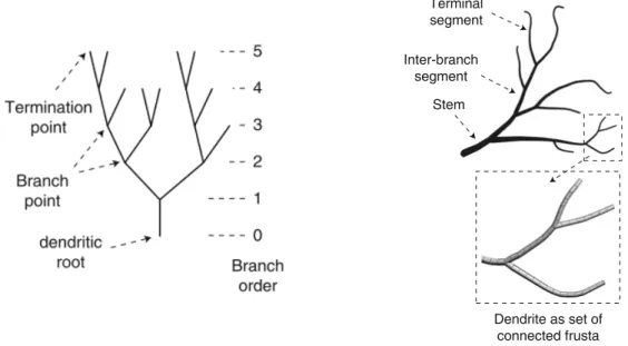
Topological analyses disregard the metric features and describe the connections in the dendritic tree structure. Quantitative description of branching structures is well developed in graph theory. A graph Γ is a pair (V, E) o a finite set V of vertices or nodes and a set E of unordered pairs, called edges or links, of different elements of V . Thus, when there is an edge e = (i, j) for i, j ∈ V , we say that i and j are connected by the edge e and that they are neighbours, i j. A special type of graph in which the edges do not form loops is called a tree, i.e., ∀e ∈ E, e 6= (i, i).

This abstract object is put in correspondence to a neuronal tree, where the three types of vertexes are the root, the branch point and the terminal tips. The two types of elements connecting the vertexes are intermediate segments and terminal segments. The root is the point of origin of the tree, located conventionally at the soma. The branch point is the vertex into which one segment enters and two or more segments exit. It is said that, at the branch point, the parent segment gives rise to two or more daughter segments. Such a branch point is called a bifurcation or multifurcation point. If all branch points of a tree are bifurcations then the tree is binary (which is the case for real dendrites). A part of the tree composed of a certain subset of connected branches and vertexes is called the subtree.

Particularly, one of the most used measures for quantitatively distinguish dendrites has been partition asymmetry that assesses the topological complexity of a neuronal tree based on the normalized difference between the degree of two daughter subtrees at a branch point. The partition asymmetry index ranges from 0 (completely symmetric) to 1 (completely asymmetric) [91]. The partition asymmetry index Ap is defined as:

Ap =

|r − s|

r + s − 2 (3.1)

with r and s indicating the number of terminal tips of each subtree, where r ≥ s, and indicates the relative difference in the number of branch points (r − 1) and (s − 1) between the subtrees. This indicator does not allow one to distinguish all the tree types of the same degree, however, other measures have even less discriminative power [64].

Measure Definition

Number of stems Total number of segments leaving from the dendritic root

Number of branch points Total number of branch points in thre tree

Branch order Topological distance from the dendritic root

Degree Termination points downstream of the node under investigation

Partition asymmetry Topological complexity of a tree

Table 3.1: List of frequently used morphometric measures to quantify neuronal topology [24].

Metrical Measures

In contrast to topological properties that have no metric interpretation, geometric properties consider the spatial embedding of a tree. Metrical parameters which characterize the