A digital image based method to quantify intracellular polyphosphates in microbial aggregates

(1)

André Paço da Fonseca

A

digital image based method to quantify intracellular

polyphosphates in microbial aggregates

(2)

(3)

André Paço da Fonseca

A

digital image based method to quantify intracellular

polyphosphates in microbial aggregates

Dissertação de Mestrado

Mestrado em Bioinformática

Trabalho realizado sob a orientação de

Investigadora Auxiliar Daniela Mesquita

Professor Doutor Eugénio Ferreira

(4)

ii

Declaração

Nome: André Paço da Fonseca

Endereço eletrónico: [email protected] Telefone: 926579490 Cartão de Cidadão: 14920072

Título da dissertação: A digital image based method to quantify intracellular polyphosphates in microbial aggregates

Orientadores:

Investigadora Auxiliar Daniela Mesquita Professor Doutor Eugénio Ferreira

Ano de conclusão. 2018 Mestrado em Bioinformática

É AUTORIZADA A REPRODUÇÃO INTEGRAL DESTA DISSERTAÇÃO APENAS PARA EFEITOS DE INVESTIGUAÇÃO, MEDIANTE DECLARAÇÃO ESCRITA DO INTERESSADO, QUE A TAL SE COMPROMETE.

Universidade do Minho, 30/11/2018

(5)

iii

Acknowledgments/Agradecimentos

Em primeiro lugar, gostaria de agradecer à minha orientadora, Daniela Mesquita, por todo o tempo que dispensou, todos os concelhos dados e pela boa disposição com que sempre se apresentou ao longo deste trabalho, o qual sem ela não seria possível de realizar. Gostaria também de agradecer ao Professor Eugénio Ferreira pela oportunidade de realizar esta tese sob o seu teto.

Gostaria de agradecer também aos colegas do LBBS por toda a simpatia e boa disposição demostrados no local de trabalho, principalmente ao Miguel Carvalho por me ter acompanhado durante todo o processo e me ter ajudado sempre que possível.

Aos meu amigos e colegas do mestrado e licenciatura, queria agradecer pela companhia durante todos estes anos, pelos risos e pelas bebedeiras, pelos jogos de futebol e kings no PDF, pelas noitadas de poker ou de conversa até de madrugada, por invadirem a minha casa mesmo sem eu saber, por me acordarem às 6 da manhã ao chegarem do enterro, por… bem, é melhor parar aqui antes que piore. Por isto tudo e muito mais, o meu mais sincero obrigado a todos vocês.

Aos colegas do 3B, que me acompanharam dia e noite durante mais de 5 anos, além de tudo o que já escrevi em cima apenas quero que saibam que vocês transformaram o 3B num verdadeiro lar e vos considero como família. Mas não, continuam a não poder fumar na sala!

À “pinguim dos montes”, obrigado por estes anos todos. Obrigado por estares comigo tanto nos bons como nos maus momentos. Evoluí imenso como pessoa, amigo, estudante e amante nestes últimos anos e muito deveu-se a ti. Obrigado!!!

Aos meus pais, agradeço por todo o esforço que fazem e sempre fizeram para me proporcionar tudo o que possa precisar, e por vezes o que não preciso também. Ao meu irmão, obrigado simplesmente por seres o meu mano mais velho, não poderia escolher melhor nem que quisesse. Ao resto da minha família, agradeço o apoio e amor incondicional que me dão.

(6)

(7)

v

Resumo

A eutrofização é um grave problema de ecossistemas aquáticos que pode ameaçar a biodiversidade e a saúde humana. É causada por uma alta concentração de nutrientes, tal como fósforo, levando a um crescimento excessivo de plantas aquáticas e, consequentemente, à estagnação e diminuição dos níveis de oxigênio nos sistemas de água.

Para evitar este problema, as águas residuais das zonas rurais, industriais e urbanas são tratadas com recurso a remoção biológica de fósforo melhorada. Esta técnica utiliza microrganismos já presentes em águas residuais que incorporam o fósforo dentro das suas células na forma de polifosfato, removendo assim o nutriente da água. Uma parte muito importante desta técnica consiste em avaliar os níveis de polifosfato presentes nos microrganismos, o que é geralmente efetuado por métodos analíticos caros e demorados.

Para melhorar a etapa de medição de polifosfatos, o objetivo desta tese foi criar um programa de análise quantitativa de imagem que pudesse correlacionar dados obtidos de imagens com dados analíticos, criando modelos de regressão linear úteis para a quantificação de polifosfatos. Este programa utilizou segmentação de cores entre regiões de polifosfato e biomassa, com base nos espaços de cores RGB, HSV e LAB, e foi aplicado em imagens de amostras tingidas com diferentes colorações (azul de metileno e azul de toluidino) e com diferentes fatores de diluição (sem diluição e diluição 10x). Estas imagens foram ajustadas nos seus valores de gamma e contraste, para avaliar diferentes configurações de imagem em segmentação de cor. Os modelos para amostras de azul de metileno e amostras diluídas apresentaram os maiores coeficientes de regressão entre os resultados dos dados de imagem e os dados analíticos (0,920 e 0,992, respetivamente), existindo também algumas diferenças entre os modelos de imagens com diferentes contrastes e valores de gamma. O espaço de cores escolhido para a análise de imagens parece ser muito importante, pois o RGB e o LAB apresentam resultados mais satisfatórios do que o HSV. Mais trabalho é necessário antes que este método possa ser usado, no entanto os resultados vistos nesta tese são promissores.

Palavras-chave: fósforo; polifosfato; remoção biológica de fósforo melhorada; análise quantitativa de imagem; azul de metileno; azul de toluidino; RGB; HSV; LAB.

(8)

(9)

vii

Abstract

Eutrophication is a serious problem of aquatic ecosystems that can threaten biodiversity and human health. It is caused by a high concentration of nutrients, such as phosphorus, leading to excessive growth of aquatic plants and, consequently, to stagnation and decreased levels of oxygen in water systems.

To prevent this problem, wastewater from rural, industrial and urban backgrounds are treated using enhanced biological phosphorous removal. This technique uses microorganisms already present in wastewater that incorporate phosphorous into their cells in the form of polyphosphate, removing the nutrient from the water. A very important part of this technique consists of evaluating the polyphosphate levels present in the microorganisms, which is usually done through expensive or time consuming analytical methods.

To improve the polyphosphate measurement step, the objective of this thesis was to create a quantitative image analysis program that can correlate image obtained data with analytical data, creating linear regression models useful for polyphosphate quantification. This program used color segmentation between polyphosphate and biomass regions, based on RGB, HSV and LAB color spaces, and was applied on images of samples dyed with different stains (methylene blue and toluidine blue) and with different dilution factors (no dilution and 10x dilution). These images experienced gamma values and contrast adjustments, to evaluate different image settings on color segmentation. Models for methylene blue stained and diluted samples presented the highest regression coefficients between the image data results and analytical data (0.920 and 0.992, respectively), also existing some differences between models of images with different contrast and gamma values.

The color space chosen for image analysis seems to be very important with RGB and LAB presenting more satisfying results than HSV. More work is needed before this method can be used, however the results seen on this thesis are promising.

Key words: phosphorous; polyphosphate; enhanced biological phosphorous removal; quantitative image analysis; methylene blue; toluidine blue; RGB; HSV; LAB.

(10)

(11)

ix

Index

Acknowledgments/Agradecimentos ... iii Resumo ... v Abstract ... vii List of figures ... xi List of Tables... xv

List of Abbreviations and Acronyms ... xvii

1. Introduction ... 1

1.1 Motivation ... 1

1.2 Objectives ... 2

2. State of the art ... 3

2.1 History of wastewater treatment ... 3

2.2 Enhanced biological phosphorus removal... 5

2.2.1 EBPR process – poly-P accumulation ... 5

2.2.2 Anaerobic phase ... 5

2.2.3 Aerobic phase ... 6

2.2.4 Phosphorus accumulating organisms (PAO)... 7

2.3 Poly-P ... 7 2.3.1 Characteristics ... 7 2.3.2 Functions ... 8 2.4 Poly-P analysis ... 8 2.4.1 Chemical analysis ... 8 2.4.2 Biological analysis ... 9 2.4.3 Molecular analysis ... 9

2.4.4 Microscopy and staining analysis ... 10

2.5 Quantitative Image Analysis (QIA) ... 11

2.5.1 Image ... 11 2.5.2 Color spaces ... 12 2.5.3 Gamma ... 14 2.5.4 Image analysis ... 15 3. Methods ... 17 3.1 Experimental set-up ... 17 3.2 Analytical procedures ... 19

(12)

x

3.4 Image analysis ... 20

3.4.1 Early script development ... 21

3.4.2 Late script development ... 21

3.5 Linear regression analysis... 23

4. Results and Discussion ... 25

4.1 Samples and images ... 25

4.2 Analytical results ... 25

4.3 QIA results ... 27

4.3.1 Early script development ... 27

4.3.2 Late script development ... 30

4.3.3 Obtained parameters... 35

4.4 Linear regression models... 42

4.4.1 Gamma and contrast... 42

4.4.2 Dye used ... 46

4.4.3 Dilution factor... 48

5. Conclusion and future work ... 53

(13)

xi

List of figures

Figure 1 Representation of the anaerobic phase biochemical reactions in a PAO. Image adapted from Tarayre [9]. ... 6 Figure 2 Representation of the aerobic phase biochemical reactions in a PAO. Image adapted from Tarayre [9]. ... 6 Figure 3 Example of poly-P linear structure. ... 7 Figure 4 Representation of the RGB color space in a three-dimensional shape – RGB cube. The x, y and z are represented with the colors red, green and blue respectively, with each coordinate representing a different color. Image adapted from Kuehni [62]. ... 12 Figure 5 Three-dimensional representation of HSV color space. HSV model is similar to a cylinder with hue (H) being arranged as a radial slice around a central axis of neutral color, saturation (S) as the horizontal depth of the structure, counting from the central axis, and value (V) as the height of the structure. This image was obtained from http://lib.povray.org and is a creative property of Michael Horvath. ... 13 Figure 6 Representation of CIELAB color space as a sphere. This image was obtained from http://sheriffblathur.blogspot.com/2013/07/cie-lab-color-space.html... 14 Figure 7 Example of data obtained on an image with QIA. Image adapted from Meijering and Cappellen [60]. ... 15 Figure 8 Representation of the lab sized bioreactor used. There were 3 tubes permanently connected to the bioreactor, namely tubes 1, 2 and 3. Tube 1 had holes at the end of it and was connected to a source of compressed air, being responsible for aeration. Tube 2 was responsible for feed, being connected to a jerrycan filled with nutrients, along with the carbon and phosphate source. Tube 3 was responsible for the discharge of the effluent. Opening 4 was usually closed, only used when a sample was taken. ... 17 Figure 9 Filtration system used during VSS and TSS analysis. ... 19 Figure 10 Representation of the RGB_mask_segmentation.m script’s workflow. ... 21 Figure 11 Representation of the Poly_P_analysis_all.m script’s workflow. The step number 1 happens before step number 2 in order to select the sample regions which will be compared to the remaining images. .. 23 Figure 12 TSS and VSS content over the experimental period. ... 26 Figure 13 Intracellular poly-P values obtained with Hach LCK 350 Phosphate Kit. ... 27 Figure 14 Intracellular poly-P values per TSS content. ... 27 Figure 15 Images obtained through microscopy (a, c and e) and their respective segmented poly-P regions (b, d and f) according to the RGB_mask_segmentation.m script using 50-180, 10-90 and 110-190 threshold values on red, green and blue bands respectively. Image a was taken on day 1, c on day 13, and e on day 29. All images were obtained from samples with no dilution, dyed with MB. Gamma and contrast settings were not altered for these images... 29 Figure 16 Images obtained through microscopy (a and c) and their respective segmented poly-P regions (b and d) according to the RGB_mask_segmentation.m script using 50-180, 10-90 and 110-190 threshold values on red, green and blue bands respectively. Image a was taken on day 1 and b on day 13. both images were obtained from samples with no dilution, dyed with TB. Gamma and contrast settings were not altered for these images. ... 30 Figure 17 Segmentation of image a into poly-P and biomass regions (b and c, respectively), when using areas 1, 2 and 3 of image a as an example of said regions plus background. The remaining pixels were assigned to each region by Euclidean distance. Images b and c were also segmented into poly-P and biomass regions (images e and f, and images h and I, respectively) with the areas assigned in image a. RGB color space was used for these images. These images were taken on day 8, MB_sd. Gamma and contrast settings were not altered for these images. ... 32 Figure 18 Segmentation of image a into poly-P and biomass regions (b and c, respectively), when using areas 1, 2 and 3 of image a as an example of said regions plus background. The remaining pixels were assigned to each

(14)

xii

region by Euclidean distance. Images b and c were also segmented into poly-P and biomass regions (images e and f, and images h and I, respectively) with the areas assigned in image a. HSV color space was used for these images. These images were taken on day 8, MB_sd. Gamma and contrast settings were not altered for these images. ... 33 Figure 19 Segmentation of image a into poly-P and biomass regions (b and c, respectively), when using areas 1, 2 and 3 of image a as an example of said regions plus background. The remaining pixels were assigned to each region by Euclidean distance. Images b and c were also segmented into poly-P and biomass regions (images e and f, and images h and I, respectively) with the areas assigned in image a. LAB color space was used for these images. These images were taken on day 8, MB_sd. Gamma and contrast settings were not altered for these images. ... 34 Figure 20 Grayscale intensity per poly-P area in RGB color space during the experimental period. Plots a-b and c-d show c-data from images with 0.8 anc-d 1.0 gamma values, respectively. Plots a-c anc-d b-c-d show c-data from images without and with contrast, respectively. ... 36 Figure 21 Grayscale intensity per poly-P area in HSV color space during the duration of the experiment. Plots a-b and c-d show data from images with 0.8 and 1.0 gamma values, respectively. Plots a-c and b-d show data from images without and with contrast, respectively. ... 37 Figure 22 Grayscale intensity per poly-P area in LAB color space during the duration of the experiment. Plots a-b and c-d show data from images with 0.8 and 1.0 gamma values, respectively. Plots a-c and b-d show data from images without and with contrast, respectively. ... 38 Figure 23 Average of poly-P area per biomass area for each day in the different gamma and contrast settings for RGB segmented images. Plots a-b and c-d show data from images with 0.8 and 1.0 gamma values, respectively. Plots a-c and b-d show data from images without and with contrast, respectively. The analytically measured intracellular poly-P concentration and intracellular poly-P per TSS are present as a red and green lines for better comparison between parameters. ... 39 Figure 24 Average of poly-P area per biomass area for each day in the different gamma and contrast settings for HSV segmented images. Plots a-b and c-d show data from images with 0.8 and 1.0 gamma values, respectively. Plots a-c and b-d show data from images without and with contrast, respectively. The analytically measured intracellular poly-P concentration and intracellular poly-P per TSS are present as a red and green lines for better comparison between parameters. ... 40 Figure 25 Average of poly-P area per biomass area for each day in the different gamma and contrast settings for LAB segmented images. Plots a-b and c-d show data from images with 0.8 and 1.0 gamma values, respectively. Plots a-c and b-d show data from images without and with contrast, respectively. The analytically measured intracellular poly-P concentration and intracellular poly-P per TSS are present as a red and green lines for better comparison between parameters. ... 41 Figure 26 Linear regression models of RGB treated images using poly-P area per biomass area as predictor variables and analytical intracellular poly-P concentration per day (left side) or per TSS (right side) as response variables. The models were created using different data based on the image settings: models A and B – G_2_C_1; models C and D – G_2_C_2; models E and F – G_4_C_1; models G and H – G_4_C_2. All image sets corresponding to their respective settings were used in the models (MB_dil, MB_sd, TB_dil and TB_sd). Data is represented as blue stars, the fitted regression line is represented in red and the model’s 95% confidence bounds are represented as light red dotted lines. The models’ regression coefficients are the following: A = 0.440, B = 0.519, C = 0.764, D = 0.655, E = 0.442, F = 0.519, G = 0.274 and H = 0.132. ... 43 Figure 27 Linear regression models of HSV treated images using poly-P area per biomass area as predictor variables and analytical intracellular poly-P concentration per day (left side) or per TSS (right side) as response variables. The models were created using different data based on the image settings: models A and B – G_2_C_1; models C and D – G_2_C_2; models E and F – G_4_C_1; models G and H – G_4_C_2. All image sets corresponding to their respective settings were used in the models (MB_dil, MB_sd, TB_dil and TB_sd). Data is represented as blue stars, the fitted regression line is represented in red and the model’s 95% confidence

(15)

xiii bounds are represented as light red dotted lines. The models’ regression coefficients are the following: A = 0.203, B = 0.202, C = 0.302, D = 0.291, E = 0.358, F = 0.450, G = 0.194 and H = 0.087. ... 44 Figure 28 Linear regression models of LAB treated images using poly-P area per biomass area as predictor variables and analytical intracellular poly-P concentration per day (left side) or per TSS (right side) as response variables. The models were created using different data based on the image settings: models A and B – G_2_C_1; models C and D – G_2_C_2; models E and F – G_4_C_1; models G and H – G_4_C_2. All image sets corresponding to their respective settings were used in the models (MB_dil, MB_sd, TB_dil and TB_sd). Data is represented as blue stars, the fitted regression line is represented in red and the model’s 95% confidence bounds are represented as light red dotted lines. The models’ regression coefficients are the following: A = 0.337, B = 0.250, C = 0.459, D = 0.283, E = 0.417, F = 0.344, G = 0.290 and H = 0.200. ... 45 Figure 29 Linear regression models of RGB treated images using poly-P area per biomass area as predictor variables and analytical intracellular poly-P concentration per day (left side) or per TSS (right side) as response variables. The models were created using different data based on the dye used: models A and B – MB; models C and D – TB. Data is represented as blue stars, the fitted regression line is represented in red and the model’s 95% confidence bounds are represented as light red dotted lines. The models’ regression coefficients are the following: A = 0.891, B = 0.824, C = 0.640 and D = 0.787. ... 46 Figure 30 Linear regression models of HSV treated images using poly-P area per biomass area as predictor variables and analytical intracellular poly-P concentration per day (left side) or per TSS (right side) as response variables. The models were created using different data based on the dye used: models A and B – MB; models C and D – TB. Data is represented as blue stars, the fitted regression line is represented in red and the model’s 95% confidence bounds are represented as light red dotted lines. The models’ regression coefficients are the following: A = 0.403, B = 0.431, C = 0.883 and D = 0.651. ... 47 Figure 31 Linear regression models of LAB treated images using poly-P area per biomass area as predictor variables and analytical intracellular poly-P concentration per day (left side) or per TSS (right side) as response variables. The models were created using different data based on the dye used: models A and B – MB; models C and D – TB. Data is represented as blue stars, the fitted regression line is represented in red and the model’s 95% confidence bounds are represented as light red dotted lines. The models’ regression coefficients are the following: A = 0.920, B = 0.919, C = 0.690 and D = 0.654. ... 48 Figure 32 Linear regression models of RGB treated images using poly-P area per biomass area as predictor variables and analytical intracellular poly-P concentration per day (left side) or per TSS (right side) as response variables. The models were created using different data based on the dilution factor: models A and B – diluted samples; models C and D – non-diluted samples. Data is represented as blue stars, the fitted regression line is represented in red and the model’s 95% confidence bounds are represented as light red dotted lines. The models’ regression coefficients are the following: A = 0.869, B = 0.978, C = 0.888 and D = 0.869. ... 49 Figure 33 Linear regression models of HSV treated images using poly-P area per biomass area as predictor variables and analytical intracellular poly-P concentration per day (left side) or per TSS (right side) as response variables. The models were created using different data based on the dilution factor: models A and B – diluted samples; models C and D – non-diluted samples. Data is represented as blue stars, the fitted regression line is represented in red and the model’s 95% confidence bounds are represented as light red dotted lines. The models’ regression coefficients are the following: A = 0.218, B = 0.429, C = 0.706 and D = 0.611. ... 50 Figure 34 Linear regression models of LAB treated images using poly-P area per biomass area as predictor variables and analytical intracellular poly-P concentration per day (left side) or per TSS (right side) as response variables. The models were created using different data based on the dilution factor: models A and B – diluted samples; models C and D – non-diluted samples. Data is represented as blue stars, the fitted regression line is represented in red and the model’s 95% confidence bounds are represented as light red dotted lines. The models’ regression coefficients are the following: A = 0.989, B = 0.992, C = 0.510 and D = 0.359. ... 51

(16)

(17)

xv

List of Tables

Table 1 Composition and concentration of nutrients that compose the synthetic feed used in the batch reactor. Trace metals composition can be seen in Table 2. This feed was based on [8], [75]. ... 18 Table 2 Composition and concentration of metals that compose the trace metals solution used in the synthetic medium. This solution is based on [8], [75]. ... 18

(18)

(19)

xvii

List of Abbreviations and Acronyms

ADP – Adenosine diphosphate AS – Activated sludge

ATP – Adenosine triphosphate C_1 – No contrast

C_2 – Higher contrast

CaCl2 · 2H2O – Calcium chloride dihydrate

CIE – Commission International d’Eclairage CoCl2 · 6H2O – Cobalt(II) chloride hexahydrate

COD – Chemical oxygen demand

CuSO4 · 5H2O – Cupric sulfate pentahydrate

DAPI – 4’,6-Diamidino-2-phenylindole dihydrochloride EBPR – Enhanced biological phosphorous removal EDTA – Ethylenediaminetetraacetic acid

FeCl3 · 6H2O – Ferric chloride hexahydrate

G_2 – Gamma value of 1 G_4 – Gamma value of 0.8 H3BO3 – Boric acid

HSV – Hue, saturation and value Int. poly-P – Intracellular polyphosphate KI – Potassium iodide

LAB – Lightness, a* and b* spaces MB – Methylene blue

MB_dil – Methylene blue diluted MB_sd – Methylene blue non-diluted

MgSO4 · 7H2O – Magnesium sulfate heptahydrate

MnCl2 · 4H2O – Manganese(II) chloride tetrahydrate

Na2MoO4 · 2H2O – Sodium Molybdate Dihydrate

NH4Cl – Ammonium chloride

NMR – Nuclear magnetic resonance OLS – Ordinary least squares

(20)

xviii

P – Phosphorous

PAO – Polyphosphate accumulating organisms PHA – Polyhydroxyalkanoates

Poly-P – Polyphosphate PPK – Poly-P kinases

P-PO4-1– Orthophosphate as phosphorus

PPX – Exopolyphosphatase QIA – Quantitative image analysis RGB – Red, green and blue SBR – Sequencing batch reactor TB – Toluidine blue

TB_dil – Toluidine blue diluted TB_sd – Toluidine blue non-diluted TCA – Tricarboxylic acid cycle TSS – Total suspended solids VSS – Volatile suspended solids

(21)

A digital image based method to quantify intracellular polyphosphates in microbial aggregates 1. Introduction

1

1. Introduction

1.1 Motivation

Water is the most important resource for human survival and life in general. There is around 1,4x109

km3 of water on Earth, however only 2,5% of the total water volume is drinkable with only a very small

percentage of this fresh water being accessible to man[1], [2]. According to the AQUASTAT database of the Food and Agriculture Organization of the United Nations, there is an estimated use of 3,9 km3 of

fresh water per year, with the greatest consumption being agriculture. Out of this amount 56% (2,2 km3)

is released into the environment as wastewater in the form of industrial or municipal effluent or agricultural drainage water. At the same time and due to increasing population, changing consumption habits, greater urbanization and industrialization, and others, water demand is predicted to increase significantly on the coming decades [3]–[5].

All these factors lead to an immense pollution of fresh water sources which can cause severe health and environmental issues, especially in poorer countries and regions. On average, high-income countries treat about 70% of wastewater, while middle-income countries treat less than 50%. Low-income countries are even worse as they treat less than 10% of their wastewater further escalating the situation for the poor who are sometimes in direct contact with polluted wastewater. It is estimated that, globally, over 80% of wastewater is released to the environment without proper treatment [3]. Although there has been an increase in wastewater treatment levels over the years, further investment and study must be made to achieve even better outcomes [6].

The lack of treatment can also directly affect ecosystems and the services they provide. Both agriculture drainage water and municipal effluent have a high concentration of nutrients such as phosphorous (P) or nitrogen that increase eutrophication of freshwater ecosystems [3]. Eutrophication is the excessive growth of aquatic plants and algae which leads to an increase in water turbidity and stagnation and to a decrease in oxygen levels, ultimately affecting wildlife in those waters [4], [7]. The removal of these nutrients from wastewater is therefore of utmost importance and it is why there are more and more wastewater treatment plants with the purpose to reduce the nutrients levels. The most common biological process for P removal, known as Enhanced Biological Phosphorous Removal (EBPR), uses microorganisms present in the wastewater to incorporate the abnormal levels of P on their cell bodies in the form of inorganic polyphosphate (poly-P). Over time the wastewater will have its phosphate concentration diminished for discharge into natural water sources [7]–[9].

(22)

A digital image based method to quantify intracellular polyphosphates in microbial aggregates 1. Introduction

2

For a proper EBPR system, fast and efficient analytical methods must be a requirement, however current poly-P monitoring techniques mostly consist of time consuming chemical methods which require prior extraction of cell’s content or other more complicated, or even more expensive methods [10]. Thus, there is an obvious need for new and faster techniques in this analytical process [8]. This thesis proposes a different approach to this problem by use of an algorithm that identifies and quantifies intracellular poly-P (int. poly-P) using images obtained with staining analysis and brightfield microscopy.

1.2 Objectives

This thesis main objective is the development of a quantitative image analysis (QIA) program that allows for the identification and quantification of poly-P inclusions in samples from an EBPR system. In detail, the technological objectives are:

1) To review relevant bibliography about poly-P and state of the art techniques and existing tools for poly-P quantification;

2) Studying and testing available relevant software tools;

3) To develop an algorithm that identifies and quantifies poly-P inclusions;

4) Compare the developed algorithm with a traditional poly-P quantification method; 5) Validation of the tool.

(23)

A digital image based method to quantify intracellular polyphosphates in microbial aggregates 2. State of the art

3

2. State of the art

2.1 History of wastewater treatment

Wastewater management has been in existence since early in the known history of mankind. In the Mesopotamian empire (3500 to 2500BC) there were drainage systems relying on storm water designed to carry away wastes into cesspools [11]. The ancient Greeks (300 BC to 500 AD) had a different approach to the problem, they used public latrines with drainage systems that collected sewage and storm water in a collection basin located outside the city which connected to nearby agricultural fields, using the wastewater for irrigation and fertilization[11]. The Romans (800 BC to 450 AD) had a strong sanitation ethic, creating a central sewer system that led wastewater into the Tiber along with aqueducts which provided clean water not only for personal use, but also for cleaning public baths, latrines and even the streets, which were used as open sewers by common people [11], [12].

With the Roman empire’s collapse so too did their sanitary ethics. Their far-reaching aqueducts were neglected and ruined over time. These sanitary “dark ages” (450 to 1750 AD) saw some attempts to properly dispose of waste and wastewater with the building of cesspools, sewers and the hiring of sanitation workers to clean the streets, however the monarchy wasn’t too concerned with the situation as long as they weren’t affected by the smell, which slowed down further development [11], [12]. In the second half of the 18th century came the industrial revolution and with it an increase in science and technology, however it was also the cause for an exponential increase in population, which worsened the already difficult situation of waste management. Due to the increasing population densities the early part of the 19th century was marked by outbreaks of diseases the likes of cholera and typhus, which is now known to be a consequence of water and waste-borne disease [11], [13]. At the time, these diseases were thought to be provoked by miasma, a type of poisoned or foul air caused by rotting waste, leading to the government placing emphasis on sanitation to prevent the spread of the disease. In London, measures such as construction of sewers and water closets helped the situation with wastewater going directly into the sewers instead of cesspools. By doing this, however, the government was unknowingly turning the river Thames into a virtual cesspool since all the sewers were connected into it [11], [13]. In 1854, Dr John Snow proved the link between water and cholera, by showing that water containing contaminated vomit or fecal matter was the cause of the disease[14]. After this the government implemented a system that collected the discharge wastewater before releasing it downriver from the city [13].

(24)

4

Only after this discovery and in the later parts of this century did people realize that pollutants needed to be removed from wastewater, which led to the first instances of wastewater treatment [11]. There were already some instances of chemical treatment in 1740, using lime as a precipitant [15], but the movement only gained favor in the mid to later stages of the 19th century. Despite its advantages, chemical treatment wasn’t completely efficient at pollutant removal and created a lot of sludge, which was difficult to dispose of [11]. The search of better treatment methods led to the creation of septic tanks and biological filters. Septic tanks consisted of large cisterns with inlets and outlets located below the surface of water, since wastewater divided itself into 3 components based on density: oils went to the top, water in the mid and settled sludge on the bottom, allowing cleaner water to be removed. It was observed that the number of solids decreased in these tanks with the passage of time, this being credited to anaerobic organisms [12], [16], [17]. Biological filters consisted of a medium used to filtrate wastewater, with porous soil being used. Wastewater that passed through sandy, gravelly soil had a decrease in pollutants, but the method later evolved into synthetic filters [16], [18]. From both methods came the idea that microorganisms could be used for wastewater treatment, which later led to extensive biological treatment research and development in the 20th century [11]. Chemical treatment was casted to the background, even though it is still used for purposes such as disinfection, chemical precipitation, neutralization and others [19].

The main biological treatment process, called activated sludge (AS), was only discovered in 1913. It was previously known that aeration of sewage allowed for oxidation of organic matter, thus diminishing the pollutants in wastewater, but it was common practice to dispose of the sludge that resulted from settling [11], [20]. In 1913, William Lockett and his team decided to aerate new portions of sewage along with previous obtained sludge. They discovered that with each aeration the amount of sludge increased and the period needed for oxidation of organic matter in the wastewater was reduced [20]– [22]. In a mere 25 years, AS was present in hundreds of full-scale wastewater treatment facilities all around the world [23]. Research into this biological process was halted until after the Second World War. From that point on the main, emphasis has been on the removal of suspended solids, organic material and nutrients, disinfection and also overall performance of the method, along with research of AS’s many variants and also anaerobic processes [11].

(25)

5

2.2 Enhanced biological phosphorus removal

EBPR was discovered in 1975 in South Africa, where its semi-arid environment, along with population growth and high chemical prices, made reuse of water essential, leading to the search of cheaper alternatives to chemical precipitants, which were, at the time, the conventional method for phosphorus and nitrogen removal [24]. EBPR is a variant of the AS process that achieves P removal by recirculating sludge through aerobic and anaerobic conditions [24]. The organisms capable of P removal are generally known as polyphosphate accumulating organisms (PAO). These incorporate P in the form of int. poly-P granules (inclusions), which leads to P removal from the liquid phase by means of cell removal in the waste AS [25].

2.2.1 EBPR process – poly-P accumulation

Poly-P accumulation doesn’t occur in anaerobic conditions; however, a single aerobic phase is not enough for efficient removal of P from wastewater. Therefore, EBPR is characterized by exposure of AS to both aerobic and anaerobic phases in cycles. Keeping in mind that oxygen can be replaced by nitrite or nitrate, the aerobic phase can be replaced with an anoxic phase or even a combination of both. This will not alter the general process of EBPR.

2.2.2 Anaerobic phase

The anaerobic phases of the EBPR process (Figure 1) are stressful for PAOs leading them to take up and accumulate carbon sources to prepare for the possibility of long-term oxygen absence. Acetate and other molecules that serve as carbon sources, such as sucrose or propionate, are thus transformed into acetyl-CoA, a reaction that consumes energy leading into the release of P, due to the hydrolysis of ATP into ADP. In this step poly-P reserves in the cell are consumed to maintain ATP levels in the cell. The accumulated acetyl-CoA is then converted and stored as polyhydroxyalkanoates (PHA), a carbon storage compound. The anaerobic phase may seem counterproductive since P is released into the medium, however, the aerobic phase intakes more than enough P to compensate [9], [26].

(26)

6

Figure 1 Representation of the anaerobic phase biochemical reactions in a PAO. Image adapted from Tarayre [9]. 2.2.3 Aerobic phase

In the aerobic phase (Figure 2), the previously stored carbon compounds, PHA, are used as fuel for cell growth and replenishment of poly-P reserves. The compounds are degraded into acetyl-CoA and enter the tricarboxylic acid cycle (TCA) cycle, which will produce the necessary energy and carbon for new cell growth. Some of the produced energy (ATP) will be used to incorporate P from the surrounding environment in the form of intracellular poly-P granules. In the aerobic stage, the microorganisms will take up almost all the surrounding P, including the one removed during the anaerobic phase. Under optimal conditions, EBPR will consume around 85% of wastewater phosphate, a great improvement to the conventional method’s 30% [9], [26].

(27)

7 2.2.4 Phosphorus accumulating organisms (PAO)

A great number of organisms can be used in EBPR as accumulators of P, from bacteria to algae and even fungi [9], however, bacteria plays the most significant role in this process. For EBPR to be efficient as a P removal method, not all PAOs can be used since the process of incorporating P intracellularly will rely mainly on the ability of the organisms present in the sludge, usually bacteria. Thus, a proper knowledge regarding the molecular mechanisms of poly-P accumulation on bacteria, and perhaps on other types of PAO, could become of help in the biological P removal from wastewater [27].

In the early beginnings of EBPR it was thought that PAOs could only accumulate P under aerobic conditions. However, based on a biological point of view, oxygen is not the only viable electron acceptor with both nitrate and nitrite being possible candidates. It is known that most bacteria possess the ability to denitrify and accumulate poly-P [28] and in fact, literature states that there is P removal in the presence of nitrate in AS systems [29], [30]. This means that there are at least two groups of PAOs, aerobic and denitrifying [28], with the latter able to remove nitrogen alongside P. Many bacteria have been reported as PAO in AS, such as: Acinetobacter, Aeromonas, Pseudomonas, Paracoccus, Bacillus, and more.[28] Acinetobacter spp. are the most common isolates found in the EBPR process, however they are not predominant, in fact several bacteria belonging to different genus are constantly being identified in EBPR processes, with both Gram-negative and Gram-positive bacteria being found.

2.3 Poly-P

2.3.1 Characteristics

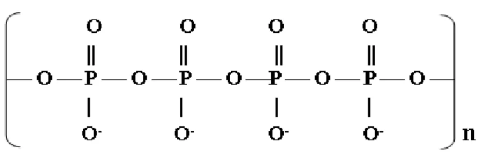
Poly-P is a linear polymer of orthophosphate residues linked by phosphoanhydride bonds, the same found in ATP. This polymer can have lengths from tens to hundreds of residues, depending on its location and metabolic state [8], [10], [31]. Due to its composition (Figure 3), it has a highly negative charge. Organic poly-P is usually found in large granules inside the cells, especially large if the organism is a PAO [25], [32].

(28)

8

2.3.2 Functions

Poly-P is a molecule with a wide range of biological functions, depending on the subcellular compartment where it is located and when it is needed. These functions include substitution for ATP in kinase reactions, regulation of enzymatic activities, capsule of bacteria, regulating some genes expressions, the physiologic adjustments to growth, development, stress and deficiency, and, with special interest to this thesis, disposal of pollutant phosphate in wastewater [33]. The biological removal of P from wastewater through poly-P production has long since been documented [4], [7], [25], [34], with poly-P serving as a high energy storage molecule that, upon hydrolysis, can supply large amounts of energy for biochemical reactions within the cell [8], however, this is not its only function in wastewater treatment since poly-P’s characteristics make it useful in other areas. Its highly negative charge, for instance, makes it helpful in preventing microbial adhesion to filter surfaces, which can prove useful in recovering microflora from drinking water [35]. Poly-P can also keep minerals in suspension during industrial processing and decrease bacterial adhesion to soil [36]. Poly-P’s reusability in wastewater treatment is yet another reason to why EBPR is the best current choice in P removal.

2.4 Poly-P analysis

Quantification and characterization of different forms of P are not easy to accomplish due to the vast uses of P in biology and its presence in several forms. Most quantification methods require a primary step to separate and concentrate the selected P fractions of interest from the rest. Poly-P can associate with other cellular components and depending on its size poly-P solubility will vary, making it a hard target for extraction [10]. Also, extraction has been reported to lead to an underestimation of poly-P values in samples owing to poly-P loss or composition change in the extraction step [37]–[39]. This implies a drop of efficiency in analytical methods with a prior extraction step, making other methods more appealing to the general scientific community.

There are several methods that enable P detection and quantification in biological sources, but not all are suitable for poly-P, with some detecting organic P or ortho-P. These methods can be divided into chemical, biological, molecular, and microscopy/staining analysis.

2.4.1 Chemical analysis

Traditional chemical poly-P quantification methods involve a digestion step to convert poly-P to ortho-P. Organic P is also converted therefore increasingly rigorous digestion methods are used to separate both types of P. The ortho-P corresponding to poly-P is then analyzed by ion chromatography or inductively

(29)

9 induced plasma atomic emission spectrometry. Since the analysis is conducted on ortho-P levels and not directly on poly-P these results may not be completely accurate due to high background ortho-P levels and the method’s own susceptibility to other P compounds [40]–[42].

High performance liquid chromatography is a very precise chemical quantification method, however it can only identify poly-P with small chain lengths, less than 35 P units, making it not compatible with the quantification of EBPR poly-P [43].

More advanced methods, such as electron ionization mass spectrometry, allow for poly-P quantification without the need of pre-extraction steps, preventing any underestimation [44].

These methods are widely used due to their cost-effectiveness and no need of advanced instruments. Still, they require work and time and are not techniques used for fast quantification of poly-P.

2.4.2 Biological analysis

Biological analysis can be divided into either enzymatic assays or protein affinity labeling. The second method can locate and visualize poly-P at the ultra-structural level tagging and detecting an epitope, the part of poly-P that is detected by the immune system [45]. This technique is not used for poly-P quantification. The first method, however, can quantify poly-P levels.

Enzymatic assays are based not on poly-P itself but on the enzymes responsible for poly-P metabolism. Poly-P is synthesized in bacteria by poly-P kinases (PPK) and degraded by exopolyphosphatase (PPX). One method involves measuring P concentration after poly-P is degraded by PPX. Another measures ATP concentration, since poly-P is converted to ATP by PPK in the presence of an excess of ADP. The reaction products can then be analyzed by chromatography, electrophoresis or other methods [37], [46], [47]. The PPK method is considered more effective for longer poly-P chains, more than 20 P units, while the PPX method seems more suited for the opposite. These techniques are highly dependent on the extraction step beforehand since they require a high poly-P purity [39].

2.4.3 Molecular analysis

Methods that pertain to molecular analysis are great non-invasive techniques that can differentiate between different species of P, such as poly-P with possible quantification. X-ray spectrometry, nuclear magnetic resonance (NMR) and RAMAN microscopy are possible molecular analysis methods for poly-P in wastewater.

When X-ray spectrometers are associated with scanning or transmission electron microscopy it is possible to directly measure the levels of elemental contents of the cells and its inclusions, such as

(30)

10

poly-P granules [48], [49]. However, quantification of environmental samples using electron microscopy is difficult, if not impossible to accomplish. There is also the possibility of fluorescence X-ray microscopy, a technique that shows the spatial concentration of elements and can be applied to poly-P. This method can only be applied to cells larger than 3 µm, making it somewhat undesirable [50], [51]. The NMR technique requires labeled substrates to operate (31P) which are included in poly-P granules

through normal cell metabolism [52]. This method allows for a good characterization of P-containing molecules, allowing for the visualization of the spectra of all P species, including poly-P. A drawback from this method is that it recognizes molecules based on their bond, meaning that other molecules that possess phosphoanhydride bonds, such as nucleotides, may interfere with poly-P detection. Also, this technique allows for a relative quantification at best, not being suitable for quantifying total poly-P levels on samples [53].

RAMAN microscopy requires a minimal sample preparation and can be used with complementary molecular techniques for better results [10]. This method has been recently used for the identification and quantification of poly-P in EBPR systems [52], however there is still no literature on this method’s ability to differentiate between poly-P’s with different chain lengths.

2.4.4 Microscopy and staining analysis

Microscopy and staining analysis involves some of the most common methods used when compound visualization and quantification is involved. These range from fluorometric to simple colorimetric techniques and provide a fast, low-cost and easy set of operations [10].

Fluorometric techniques involve staining of poly-P granules with specific fluorescent dyes. The most common fluorescent staining method for poly-P detection uses 4’,6-Diamidino-2-phenylindole dihydrochloride (DAPI) [54], [55]. This dye is not specific to poly-P, staining DNA as well as other compounds, but this behavior can be circumvented with high enough concentrations of DAPI, with DNA-DAPI turning blue while poly-P-DNA-DAPI yellow [39], [54], [56]. Methods for quantification of poly-P using DAPI have already been created with promising results [8], [55].

Intracellular poly-P granules are not visible through an optical microscope, unless stained which led to colorimetric methods in poly-P visualization and quantification. These methods were the first to be implemented and are still widely used due to their simplicity. They consist of staining biomass with chemicals (dyes) and observing them through a brightfield microscope [9]. There are two major stains commonly used in EBPR studies, Neisser and Loeffler staining, and both use Methylene Blue (MB) as

(31)

11 their active component. This dye can be replaced with Toluidine Blue (TB), which shares similar properties, and can also be used for poly-P staining. MB is a metachromatic dye with a high positive charge that has a high affinity for poly-P granules, due to their anionic properties. When this dye binds to poly-P it produces a color different from the rest of the cell, allowing for the differentiation between them through microscopy [57], [58]. These dyes alone are already enough for poly-P differentiation, with Loeffler and Neisser methods further increasing the visual difference between cell and poly-P granules.

Loeffler’s method has been reported to have a higher efficiency towards larger poly-P granules, with good results in EBPR systems with large poly-P quantities [57]. Through this method, pink-violet poly-P granules are seen amidst a blue background corresponding to the cells [59].

When using Neisser staining method, MB is dissolved in an acidic solution that helps better differentiate poly-P granules and the rest of the cell since MB only binds to molecules with lower pH than the solution, which is the case of poly-P. Afterwards a counterstain solution is added. This method makes Neisser staining more suitable for poly-P staining than Loeffler’s since it provides a better contrast between poly-P and the cell. Through this method, purple-black poly-P granules are seen amidst a yellow-brown background corresponding to the cells [57].

In EBPR systems, cell staining after the aerobic phase with any of these methods, should show the entire cell as stained instead of individual granules, due to large amounts of poly-P present in PAO [32].

2.5 Quantitative Image Analysis (QIA)

2.5.1 Image

An image may be defined as a two-dimensional function, f (x, y), where x and y are spatial coordinates, and the amplitude in any given coordinate (pixel) is the intensity of the image at that point. When f, x and y are finite and discrete quantities, the image is a digital image. In monochrome images, the intensity value of pixel is usually known as gray level, since the variation between black and white is what enables us to see a picture. Mathematically speaking, images are n-dimensional matrices (with n typically 1-5) with each dimension corresponding to a different parameter or coordinate [60]. For example, in the RGB (red, green and blue) color system, an image consists of three individual monochrome images, each corresponding to their respective color [61]. The junction of these three individual monochromatic images is the original color image.

(32)

12

2.5.2 Color spaces

A color can be represented through a series of different mathematical systems. These are called color spaces or color models, and each possess different qualities that enables them to better perform certain tasks when compared to each other.

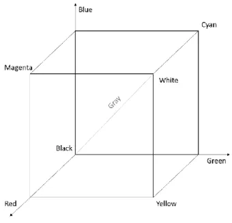
RGB is the most common color system, but it’s not the only one, in fact there are several of these color spaces, such as HSV or CIELAB, which are mathematical representations of sets of color [62]. In RGB color space there are three primary colors: red (R), green (G), and blue (B), that added together can form all other colors including black and white. This model is usually represented as a cube due to the models three main colors (Figure 4), which act as the axis for the model. RGB values are conventionally normalized to range from 0 (not saturated) to 1 (fully saturated), however they can also be represented in an 8-bit system, ranging from 0 (not saturated) to 255 (fully saturated) [63].

Figure 4 Representation of the RGB color space in a three-dimensional shape – RGB cube. The x, y and z are represented with the colors red, green and blue respectively, with each coordinate representing a different color. Image adapted from Kuehni [62].

The simplicity and versatility of this color space makes it the most common choice for computer graphics, however RGB is not very efficient when dealing with “real-world” images so other color systems were designed [62], [63]. One color space that takes human perception and interpretation of color into account is HSV (hue, saturation, and value), among others. It was designed to be more intuitive in manipulating color in a time when color had to be specified manually in systems. This color model allowed for a simplification of programming, processing, and end-user manipulation processes, making it suitable for color manipulation such as color identification and segmentation. This color space

(33)

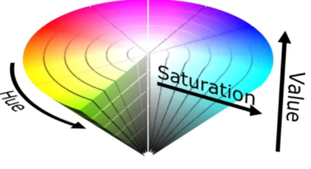
13 is usually represented as a cylinder or as a cone (Figure 5) [62]. Unlike RGB this color space doesn’t have the same range of values in its “dimensions”. Hue (H) refers to the basic color and is defined as the angle around the color plane from a reference to the specific color, ranging from 0 (red) to 360 (also red, since it’s a circle). Saturation (S) and value (V) are defined as the departure of the color from white and black, respectively, and are defined as two vectors, with saturation being the distance between the central circle point and the specific pure color, and value being the vertical position where the circle plane intersects the grey vertical axis. Both saturation and value conventionally possess normalized values ranging from 0 (white or black) to 1 (specific color), or as a percentage.

Figure 5 Three-dimensional representation of HSV color space. HSV model is similar to a cylinder with hue (H) being arranged as a radial slice around a central axis of neutral color, saturation (S) as the horizontal depth of the structure, counting from the central axis, and value (V) as the height of the structure. This image was obtained from

http://lib.povray.org and is a creative property of Michael Horvath.

Another important color space and presently the most important system of color representation is the CIELAB model, also called LAB or L*a*b. Created by the Commission International d’Eclairage (CIE) in 1976, this model is a result of several years of study and development and is based on the opponent color theory. Designed to be perceptually uniform with respect to human color vision and considered one of the most accurate color systems in the organization of colors, this 3D model is composed of three different axes: a vertical L* axis, that relates to the luminance of the color and ranges from black to white and two perpendicular horizontal axis, a* and b* which range from red to green and yellow to blue, respectively [63]. Conventionally, red and yellow are positive on their axes with values up to +154 while green and blue are negative with values down to -155 (8-bit integer). L values range from 0 (darker) to 100 (lighter). This relates to the fact that it’s considered impossible for any color to be both green and red, or yellow and blue at the same time, according to the opponent color theory [64]. This color space is usually represented as a sphere (Figure 6).

(34)

14

Figure 6 Representation of CIELAB color space as a sphere. This image was obtained from

http://sheriffblathur.blogspot.com/2013/07/cie-lab-color-space.html.

All these color spaces are interchangeable, which allows for an easy transformation of a RGB image to HSV, LAB or others, and even vice-versa, through the use of mathematical equations [62], [63].

2.5.3 Gamma

Another important element when dealing with images is gamma correction, or simply gamma. While it is not directly related to color, it can significantly change the perception of colors and brightness of an image.

The intensity of light generated by a physical device is not a linear function of the applied signal, instead being the approximate applied voltage raised to a gamma power. If an image was stored in a linear manner, instead of gamma encoded, it would use an excess number of bits to describe brighter tones due to the higher sensitivity of cameras on this tonal range. Gamma increases the visual quality of an image since humans perceive color and brightness in a nonlinear manner. Gamma correction, which is a simple altering of the gamma value, is therefore a nonlinear operation that optimizes the usage of bits, giving more importance to shadow values that humans are more sensitive to or to highlights that humans cannot differentiate, depending on the purpose of the correction. To put it simply, gamma values define how much dark colors are highlighted in an image. Higher gamma values will darken shadows and darker regions, while lower gamma values will do the opposite, brightening those areas [62], [65].

(35)

15 2.5.4 Image analysis

Image analysis is defined as the act of measuring meaningful object features in an image, with these objects being colors, sections or others (Figure 7). The results can be qualitative or quantitative with a tendency for quantification in most fields of research [60].

QIA techniques are becoming increasingly more important in many scientific fields, with a great focus on biology. The increase in both image hardware acquisition efficiency and data storage and processing, along with a need for faster and less subjective approaches has made QIA techniques indispensable and increasingly needed in science [60]. There are numerous QIA methods, adapted for their specific needs, but some steps are common in those methods, such as pre-treatment of images, filtering, and segmentation [66]–[68].

Figure 7Example of data obtained on an image with QIA. Image adapted from Meijering and Cappellen[60].

QIA methods have recently been used to obtain valuable information about biological processes, being applied for content and morphology determination in EBPR biomass using bright-field, phase-contrast, and/or fluorescence microscopy [69]–[72].

Despite their uses in microorganism or intracellular storage compounds identification (poly-P, PHA, glycogen) [58], [73], these processes are generally not used in routine quantitative analysis, being overshadowed by other more widespread and influential methods, such as chromatography. This implies a need for the development of even more QIA algorithms and techniques in EBPR systems but also on other fields of study.

(36)

(37)

A digital image based method to quantify intracellular polyphosphates in microbial aggregates 3. Methods

17

3. Methods

3.1 Experimental set-up

Experimental results were obtained in a laboratory-scale sequencing batch reactor (SBR) with a working volume of 4L (Figure 8) operated for 29 days. In this experiment, synthetic wastewater was used with acetate as main carbon source and dipotassium phosphate as phosphate source. The chemical oxygen demand (COD)/P ratio was originally planned to slowly decrease from 27 mg COD per mg P-PO4-1 to 10

mg COD per mg P-PO4-1 to provide advantages to PAO [8], [74], unfortunately phosphate was not

dissolving properly below 20 mg COD per mg P-PO4-1 so this ratio was kept throughout the duration of

the experiment.

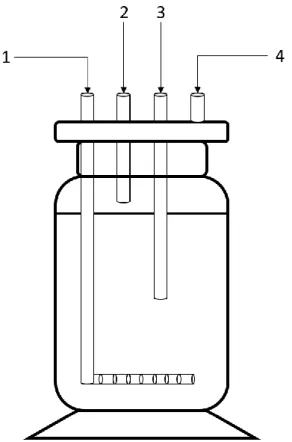
Figure 8 Representation of the lab sized bioreactor used. There were 3 tubes permanently connected to the bioreactor, namely tubes 1, 2 and 3. Tube 1 had holes at the end of it and was connected to a source of compressed air, being responsible for aeration. Tube 2 was responsible for feed, being connected to a jerrycan filled with nutrients, along with the carbon and phosphate source. Tube 3 was responsible for the discharge of the effluent. Opening 4 was usually closed, only used when a sample was taken.

Synthetic feed consisted of the carbon and phosphate source along with other key nutrients according to [8], [75]. Their composition can be found in Table 1. Trace metals solution was created separately and then added to the synthetic feed. Their composition is seen in Table 2.

(38)

18

Table 1 Composition and concentration of nutrients that compose the synthetic feed used in the batch reactor. Trace metals composition can be seen in Table 2. This feed was based on [8], [75].

Synthetic feed (gL-1) NH4Cl 0,59 MgSO4 · 7 H2O 0,95 CaCl2 · 2 H2O 0,44 Allyl-N thiourea 0,012 EDTA 0,03 Trace metals 3.16 mLL-1

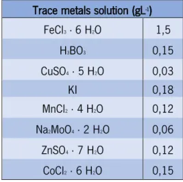
Table 2 Composition and concentration of metals that compose the trace metals solution used in the synthetic medium. This solution is based on [8], [75].

Trace metals solution (gL-1)

FeCl3 · 6 H2O 1,5 H3BO3 0,15 CuSO4 · 5 H2O 0,03 KI 0,18 MnCl2 · 4 H2O 0,12 Na2MoO4 · 2 H2O 0,06 ZnSO4 · 7 H2O 0,12 CoCl2 · 6 H2O 0,15

The system operated with the help of electronic timers, with a cycle of 6h consisting of 120 min anaerobic including 45 min feed, 180 min aerobic, and 60 min settling including 5 min wasting. One on/off control valve was used, bubbling compressed air into the reactor during aerobic periods. The pH was periodically monitored to ensure that it remained around 7.5.

Samples were obtained from the bioreactor immediately after the end of the aerobic period. Samples were also diluted in a 1/10 ratio, with both the diluted and non-diluted samples being stained for posterior image analysis. The remaining samples were stored at -20ºC for posterior analytical procedures.

(39)

19

3.2 Analytical procedures

Poly-P content, total suspended solids (TSS), and volatile suspended solids (VSS) were always analyzed at the end of the aerobic stage using the same samples used for staining and image acquisition. Poly-P content was measured using a Hach LCK 350 Phosphate Kit. This kit has two different protocols, one for measuring dissolved orthophosphate (a) and the other for measuring the total P (b) content of the sample. The orthophosphate procedure involves adding 0.5 ml of Reagent B to 0.4 ml of sample on a cuvette and closing it with a DosiCap C. The cuvette is then inverted 2 to 3 times so that the cap’s frozen content is dissolved. After 10 minutes the sample is ready for analysis. The total P procedure involves a prior hydrolysis step, with DosiCap Zip content and 15 minutes at 170ºC using a HT 200 S, before following the same procedure as the orthophosphate analysis. Poly-P concentration was calculated by subtracting the dissolved orthophosphate from the total P content (Poly-P=b-a).

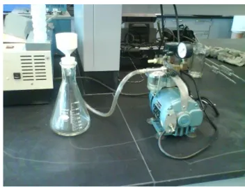
TSS and VSS were measured using the standard methods [76]. Glass fiber filters were placed on top of an aluminum dish and weighted (a). Afterwards, 5 ml of sample (V) was filtered using a standard filtration system (Figure 9). The biomass filled filters, along with the aluminum dish, were heated at 105ºC for 24h. They were weighted again after cooling down (b). These were then reheated at 550ºC during 2h for removal of volatile substances. All that remains in the filters is inorganic matter, usually referred to as fixed solids. The filters were then weighted again after a cooldown period (c). The TSS and VSS were calculated using Equation 1 and Equation 2, respectively, and expressed in gL-1.

Figure 9 Filtration system used during VSS and TSS analysis.

𝐓𝐒𝐒 = (𝐛 − 𝐚) × 𝟏𝟎𝟎𝟎/𝐕 Equation 1

(40)

20

3.3 Staining and image acquisition

Intracellular poly-P inclusions were observed using standard brightfield microscopy at 20 times magnification with MB and TB staining. To keep the process simple, the dyes were used without any additives, as sent by the manufacturer (MB’s manufacturer was CONDA Labs while TB’s was PanReac). The staining method used was simple: around 0.5 ml of sample was put on top of a slide and spread carefully. The sample was dried at room temperature, after which it was covered with dye for no more than 30 seconds and washed with distilled water immediately after. After drying at room temperature once again, the sample was ready for visualization.

This method was also used for diluted samples with a 1/10 ratio. This dilution was used to prevent biomass overlapping during image visualization. Images were then acquired from all four stained slides thus obtaining 4 sets of around 50 images each: MB diluted (MB_dil), MB non-diluted (MB_sd), TB diluted (TB_dil), and TB non-diluted (TB_sd). Images were obtained using an Olympus BX51 optical microscope (Olympus, Tokyo, Japan), coupled with an Olympus DP72 camera (Olympus, Tokyo, Japan). Images were acquired at 1360 × 1024 pixels through the commercial software CellˆB (Olympus, Tokyo, Japan). Images were then analyzed with the help of a MATLABTM written image

analysis algorithm.

3.4 Image analysis

The algorithms developed in this thesis were created using solely MATLAB R2015. The image processing and analysis were based on the identification of poly-P regions, be they intracellular inclusions or other (aggregated, superimposed regions or even ruptured granules), through color segmentation. There are several mathematical representations of color, called color spaces, but for this thesis three were chosen for the color segmentation process: RGB, HSV, and LAB. They were chosen due to their different qualities and their differences in organizing color as to select the most appropriate color space for this work. The mechanism through which color segmentation was performed was basically the same for all color spaces, dividing each image into three different areas representing poly-P, biomass, and background. Two different gamma values and contrast settings were used in an attempt to better visualize the different colors and perform correct segmentation for posterior data analysis. Images obtained by microscopy were organized by day, dye used, and dilution factor, for faster analysis.

(41)

21 3.4.1 Early script development

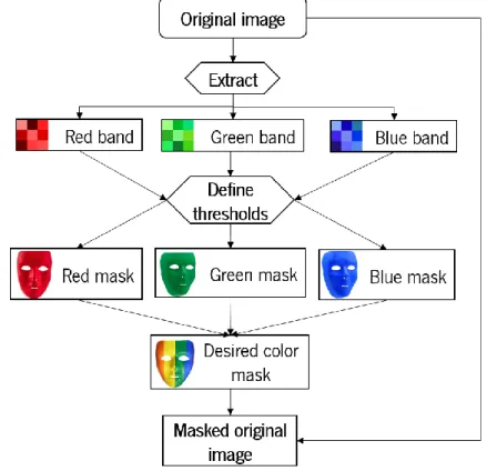
There was an evolution in terms of scripts used during this thesis. A sort of trial and error methodology was applied, with scripts being created and discarded if they did not correspond to expectations or where deemed too difficult to use. Early in this thesis, a script called RGB_mask_segmentation.m, was created for color segmentation. This script operated on the basis of thresholding RGB values on the obtained microscopy images. The RGB images were divided into their three color bands, onto which a low threshold and a high threshold were designed. The image pixels with values that ranged between both thresholds were used to create color masks while the other pixels were discarded. These masks were then applied in their respective color band creating masked images for each band, or simply put, images corresponding to each color band with their desired values. The combination of all three masked images create a colored mask which, when applied on the original image, led to the final image showing the desired color. The workflow for this script can be seen in Figure 10.

Figure 10 Representation of the RGB_mask_segmentation.m script’s workflow. 3.4.2 Late script development

The final two types of scripts used were Poly_P_analysis_all.m, a script that utilizes the three color spaces to segment sets of images on the three different regions and saves the data extracted from them on an excel file, and x_color_separation.m, where x stands for HSV, RGB, or LAB, which are