Journal Pre-proofs
A Density-Peak-Based Clustering Algorithm of Automatically Determining the Number of Clusters
Wuning Tong, Sen Liu, Xiao-Zhi Gao
PII: S0925-2312(20)31676-3
DOI:
https://doi.org/10.1016/j.neucom.2020.03.125Reference: NEUCOM 22980
To appear in:
NeurocomputingRevised Date: 4 February 2020 Accepted Date: 23 March 2020
Please cite this article as: W. Tong, S. Liu, X-Z. Gao, A Density-Peak-Based Clustering Algorithm of Automatically Determining the Number of Clusters,
Neurocomputing (2020), doi: https://doi.org/10.1016/j.neucom.2020.03.125
This is a PDF file of an article that has undergone enhancements after acceptance, such as the addition of a cover page and metadata, and formatting for readability, but it is not yet the definitive version of record. This version will undergo additional copyediting, typesetting and review before it is published in its final form, but we are providing this version to give early visibility of the article. Please note that, during the production process, errors may be discovered which could affect the content, and all legal disclaimers that apply to the journal pertain.
© 2020 Published by Elsevier B.V.
A Density-Peak-Based Clustering Algorithm of Automatically Determining the Number of Clusters
Wuning Tonga,b,∗, Sen Liua, Xiao-Zhi Gaoc
aSchool of Computer Science and Technology, Xidian University, Xi’an,710071, China
bDepartment of Science and Technology, Shaanxi University of Chinese Medicine, Xianyang, 712046, China
cSchool of Computing, University of Eastern Finland, Kuopio, Finland
Abstract
Clustering is a typical and important method to discover new structures and knowledge from data sets. Most existing clustering methods need to know the number of clusters in advance, which is difficult. Some algorithms claim they do not need to know the number of clusters in advance. Among these algorithms, however, some need to manually determine the cluster centers in a decision graph, which is not easy; some assume that the number of initial cluster centers given is greater than the actual number of classes, but in fact the true number of clusters is not known. In order to tackle this issue, we propose a density- peak-based clustering algorithm of automatically determining the number of clusters. First, we design a density metric by using a continuous function which can well distinguish the densities of different data points. Then, we design a pre- clustering method which can get the initial cluster centers and the corresponding clusters. Furthermore, we propose an automatic clustering method which can automatically determine the final cluster centers and the corresponding clusters.
Experiments are conducted on widely used data sets, and the results show the effectiveness of the proposed method.
Keywords: Clustering, Automatic determination of the number of clusters, Density peak, Cluster centers merging
∗Corresponding author
Email address: [email protected](Wuning Tong)
1. Introduction
With the quick development of the Internet and information technologies, we are facing the challenge of processing increasing amounts of data. How to discov- er new structures and new knowledge from these data is an urgent issue. Clus- tering is an unsupervised learning method which does not need prior knowledge
5
[1, 2]. Today, clustering algorithms have been widely used to find the internal structure of the medical [3, 4, 5], academic [6, 7], commercial[8, 9], and traffic data [10, 11, 12] etc., and to serve as the fundamental and preparatory step before more advanced functionalities such as recognition of images[13, 14, 15], segmentation of texts[16, 17] and discovery of communities[18] are implemented.
10
Traditional clustering algorithms can often be classified into five types [19, 20, 21]: partitioning clustering algorithms, hierarchical clustering algorithm- s, density-based clustering algorithms, grid-based clustering algorithms, and model-based clustering algorithms. The K-means algorithm is a representative of the partitioning clustering algorithms [22]. It is simple and fast when the
15
data’s distribution is close to the Gaussian distribution, but it is sensitive to noise points and outliers in the data set. The W-k-means algorithm[23] can au- tomatically calculate the weight of the variables, remove the noise points that affect the clustering result in the clustering process, and thus obtain a better clustering result. However, these K-means type clustering algorithms [22, 23, 24]
20
need to specify the number of clusters in advance, and the choice of the initial cluster centers has a greater impact on the clustering result. Furthermore, they tend to find the spherical clusters with similar scales and densitys, and do not work well for non-convex data clusters. The algorithm BIRCH is a representa- tive of the hierarchical clustering algorithms [25, 26]. BIRCH uses less memory
25
and less computing time, and can effectively identify noise points. However, this algorithm also needs to know the number of clusters in advance, and need- s to pre-assign some parameters such as the radius threshold and number of features in the non-leaf nodes and the leaf nodes. These parameters have a great influence on the number of clusters and clustering results. Unreasonable
30
parameter setting will result in incorrect clustering results. In addition, the BIRCH algorithm does not work well for non-convex data clusters. DBSCAN is a representative of the density-based clustering algorithms [27, 28]. It can find spatial clustering of arbitrary shapes and does not need the number of clus- ters in advance, but it needs additional parameters (e.g., neighbor radius Eps
35
and minimum number of samples in the neighborhood MinPts), which have a great influence on the clustering result. Furthermore, these parameters need to be tuned individually for different data sets. Additionally, DBSCAN does not work well for high-dimensional data. STING is a representative algorithm of the grid-based methods [29]. Its processing time is independent of the number
40
and input order of data. It can process any type of data, but the processing time depends on the number of cells divided in each dimension space, which reduces the quality and accuracy of clusters to some extent. COBWEB, a typi- cal model-based algorithm [30], expresses clusters in the form of a classification tree. It is sensitive to the order of data input, and the probability distribution
45
and storage of clusters are quite complicated.
Most existing methods in these 5 types need to know the number of clusters in advance, but more often we do not know the number of clusters in advance.
There have been some algorithms claiming they do not need to know the number of clusters in advance. For examples, RPCL [31], which belongs to the parti-
50
tioning clustering algorithm, first arranges the number of seeds greater than the actual number of clusters, and automatically determines the number of clusters by driving the extra seeds away from the dense regions based on the delearning rate. However, the algorithm is sensitive to the delearning rate, and improper delearning rates will induce incorrect clustering results. To overcome this short-
55
coming, RPCCL [32] adds a mechanism to dynamically control the strength of the rival penalization and decrease the effect of the delearning rate. Recently, RP-WOCIL[33] used the rival penalty mechanism to automatically acquire the initial cluster centers. However, these algorithms assume that the number of initial cluster centers given is greater than the actual number of classes, but in
60
fact the true number of clusters is not known. If the number of seeds is too large,
the computation cost will increase greatly. FSFDP [34] (Fast Search and Find of Density Peaks), a density-based clustering algorithms, published in Science in 2014, also claimed that it did not need the number of clusters in advance. It is observed that the local densities of cluster center points are relatively large,
65
and their distances to other cluster centers are also relatively large. According to this observation, the cluster centers are selected manually, and then other data points are classified into the cluster whose center is the nearest to these data points. However, it is hard to manually select cluster centers on the deci- sion graph, especially for data sets which do not have clear boundaries among
70
clusters, and the cluster results will be greatly affected by the manual selection of the cluster centers.
To overcome the above problems, in this paper, we propose a new cluster- ing algorithm called Density-Peak-Based Clustering Algorithm of Automatically Determining the Number of Clusters (briefly DPADN). The proposed algorithm
75
first uses a continuous function to calculate the densityρ, and employs the same method as that in FSFDP [34] to calculate the distanceδfor each data point to generate a decision graph. Then we design a pre-clustering method which can get the initial cluster centers and the corresponding clusters from the decision graph. After that we propose an automatic clustering method which can au-
80
tomatically determine the final cluster centers and the corresponding clusters.
To realize this, we first compute the distances between every two initial cluster centers and sort the distances in ascending order. Then we find the smallest dis- tance in the queue which corresponds to the two cluster centers nearest to each other currently and merge the two corresponding initial clusters into one, but
85
still keep the two cluster centers in the merged cluster (i.e., the merged cluster has one additional cluster center). After that, we delete the smallest distance in the queue. This merging process repeats until only one cluster is left. The number of clusters which is kept unchanged for the most merging times is the final number of clusters and the corresponding clusters are the final clusters by
90
the Scale Space Theory of the visual system[35, 36]. Finally, experiments are conducted on ten data sets and the results show the effectiveness of the proposed
method.
The main contributions of our work are as follows:
1. We have designed an algorithm for automatically acquiring cluster centers
95
and the corresponding clusters.
2. We have designed a scheme for selecting the initial cluster centers, which excludes noise points to reduce the influence of noise points on clustering.
3. We have improved the density calculation method by using a continuous function, which can well distinguish the densities of different data points.
100
The remainder of the paper is organized as follows: Section 2 reviews the related work. Section 3 describes the proposed algorithm in detail. Section 4 shows the experiment results, and conclusions are drawn in Section 5.
2. Related Work
2.1. Algorithm FSFDP
105
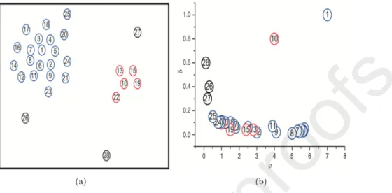
The main idea of FSFDP [34] is that a cluster center should be surrounded by data points that do not exceed its density and be relatively far away from the data points that are denser than it. For this purpose, FSFDP constructs a decision graph based on the densityρand the distanceδ, and manually selects the points with a relatively large distance δ and density ρ as cluster centers.
110
Suppose there is a data setS={xi}ni=1withnsamples andmdimensions. Let di,j represent the Euclidean distance between the data pointsxi andxj:
di,j= v u u t
m
X
t=1
(xti−xtj)2. (1)
The density of thei-th data point is calculated with the Cut-off kernel func- tion as follows:
ρi=X
j6=i
X(dij−dc) (2)
where dc represents the distance threshold, X(x)=1 if x < 0 and otherwise
115
X(x)=0. In [34],dcis assigned a specific value to make the average number of neighbors around 2% of the total number of objects in the data set. Therefore, ρi means the number of data points whose distances from the point i are less than dc. For the data point with the highest density, the distance δ is the maximum value of all distances among the data point pairs. For any other data
120
point, the distance δ is the minimum value of all the distances from it to all the data points that are denser than it. The distance of data point xi can be calculated in two cases as follows:
δi=
j:ρmaxi>ρj
(dij) if∀j s.t.ρj≤ρi j:ρminj>ρi
(dij) otherwise
(3)
By using the density and distance as the abscissa and the ordinate, respec- tively, FSFDP generates a decision graph. Figure 1 is an example of the decision
125
graph for two dimensional data, where Figure 1(a) shows two clusters represent- ed with different colors and Figure 1(b) is the decision graph where Points 1 and 10 have a larger density and distance than others and therefore are the cluster centers. Points 26, 27 and 28 have a larger distance but a smaller density, so they are considered as noises. After determining the cluster centers and noises,
130
the remaining data points can be assigned to its nearest cluster [34].
2.2. The Scale Space Theory
For a data set, when we observe it at different distances (i.e., using different length scales), we may obtain different clusters (different numbers and centers of clusters). For example, when we observe it very far away, we may see that
135
all of the data are clustered together and thus form a single cluster. But when we observe it very near, we may see that all of the data are separated and thus each data forms a cluster. This means that the cluster results (the number of clusters and the centers of the clusters) of a data set may be different with different distance scales on which we observe the data set. However, in practical
140
(a) (b)
Figure 1: FSFDP data set and its decision graph
applications, only when we observe the data set from a proper distance scale, can we obtain correct clusters. To address this issue, we can use the Scale Space Theory [37, 38].
The Scale Space Theory is a theory to study the perception of the minimum change of the stimulation intensity by the visual system. It has a property called
145
the scale-invariant property, that is, when a person recognizes an object, he can correctly identify it within a certain distance range [37, 38]. This is because the main features and the structure of the object can be observed in this range. It can be used in clustering to obtain a proper clustering result.
Witkin[39] conducted a series of tests and concluded that we could obtain
150
the unchanged visual information (unchanged main features) of the observed ob- ject when we constantly change the observation distance within a certain range.
The larger the variation of the observation distance in this range, the more im- portant the obtained visual information, and using the maximum variation of the observation distance in this range can help us to obtain the main features of
155
the observed object most exactly. Later, Weber drew an important conclusion called Weber’s Law [40]. According to it, the minimum change ∆I in the s- timulus intensity perceived by the visual system is proportional to the standard
stimulus intensity I, i.e., ∆I= kI, where k is a positive constant. When the actual change in the stimulus intensity satisfies ∆I′ < kI, there is no change
160
in the visual system (i.e., we cannot feel any change in the observed object). If the stimulus intensity is represented by the size (scale) of the observed object (directly related to the distance from the observed object)S, the minimum scale change ∆S on the object that can be perceived is proportional to the sizeS of the object, as shown in Equation(4):
165
∆S=kS (4)
wherekis a positive constant with the value in the range between 0.03 and 0.07 [40]. When the actual scale change satisfies ∆S′ < kS, we do not perceive any visual change in the object. The larger the ∆S′, which results in no feel of the visual change, the more representative the main features of the object observed.
We can use Weber’s Law to determine the number of clusters. The idea is as
170
follows: if we observe a data set with constantly changing distances (constantly changing visual perception of the size or scale of the object), the number of clusters and clusters themselves will change constantly. Based on Weber’s Law, the number of clusters and the clusters themselves of the data set which remain unchanged for the most merging times will be the final number of clusters and
175
the clusters.
2.3. Agglomerative Hierarchical Clustering
Hierarchical Clustering is a common clustering algorithm. It creates a hierar- chical clustering tree by calculating the similarity between different data points.
In the clustering tree, the original data points are the nodes in the bottom layer
180
of the tree (leaf nodes), and the top layer of the tree is the root node. There are two methods to create a clustering tree: the bottom-up (agglomerative) method and the top-down(divisive) method. Hierarchical clustering methods can be further divided into agglomerative (aggregative) hierarchical clustering and divisive hierarchical clustering. The Agens[41] algorithm belongs to the
185
first type. It can find the hierarchical relationship of the data set and can be described in the following Algorithm 1.
Algorithm 1The Agens algorithm.
Input: data setS={x1,x2,· · ·,xn}, cluster number K Output: cluster labelC={c1,c2,· · ·,cn}
1: fori= 1to n do
2: ci=xi;
3: end for
4: Calculate the distance between any two points in the data set S;
5: Set the current number of clustersnum=n;
6: whilenum > K do
7: Find the two nearest clusters ci andcj;
8: merge these two clusters into a new cluster;
9: Recalculate the distance between the new cluster and each of others clusters;
10: num=num−1;
11: end while
However, the Agens[41] algorithm still needs to assign an expected number K of clusters in advance and recalculate the distance between the new cluster and each of the other clusters. Therefore, it has quite a high computational
190
cost.
3. Density-Peak-Based Clustering Algorithm of Automatically De- termining the Number of Clusters(DPADN)
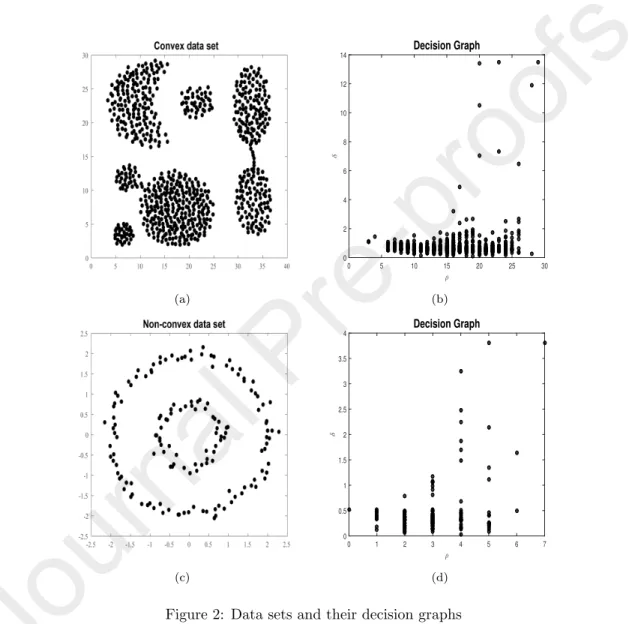
FSFDP[34] needs to select cluster centers manually from the decision graph, which is not easy in many applications. The Aggregation data set and Double-
195
circles data set are two typical examples of the widely used data sets, whose data distribution and decision graph are shown in Figure 2.
We can see from Figure 2(a) that this data set is a convex data set and has seven clusters. Similarly, the data set in Figure 2(c) is a non-convex data set and has two clusters. For both data sets, it is difficult to manually select
200
accurate cluster centers from the decision graph, as demonstrated in Figures 2(b) and (d). To address this problem, we propose a new clustering algorithm which can automatically acquire the cluster centers.
(a)
ρ
0 5 10 15 20 25 30
δ
0 2 4 6 8 10 12 14
Decision Graph
(b)
(c)
ρ
0 1 2 3 4 5 6 7
δ
0 0.5 1 1.5 2 2.5 3 3.5
4 Decision Graph
(d)
Figure 2: Data sets and their decision graphs
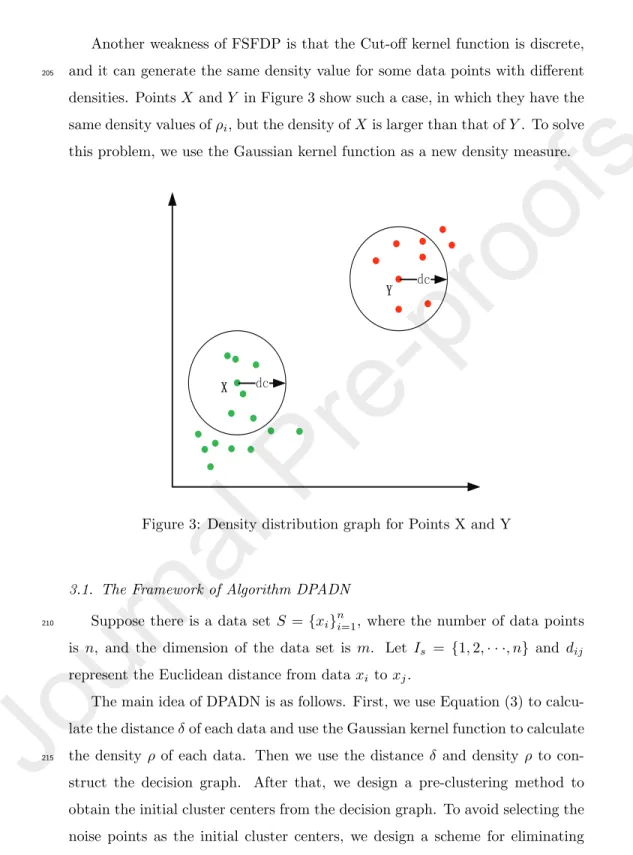
Another weakness of FSFDP is that the Cut-off kernel function is discrete, and it can generate the same density value for some data points with different
205
densities. PointsX andY in Figure 3 show such a case, in which they have the same density values ofρi, but the density ofX is larger than that ofY. To solve this problem, we use the Gaussian kernel function as a new density measure.
GF
GF
Figure 3: Density distribution graph for Points X and Y
3.1. The Framework of Algorithm DPADN
Suppose there is a data setS ={xi}ni=1, where the number of data points
210
is n, and the dimension of the data set is m. Let Is = {1,2,· · ·, n} and dij
represent the Euclidean distance from dataxi toxj.
The main idea of DPADN is as follows. First, we use Equation (3) to calcu- late the distanceδof each data and use the Gaussian kernel function to calculate the densityρ of each data. Then we use the distanceδ and density ρ to con-
215
struct the decision graph. After that, we design a pre-clustering method to obtain the initial cluster centers from the decision graph. To avoid selecting the noise points as the initial cluster centers, we design a scheme for eliminating
noise points in the pre-clustering method. After we have determined the initial cluster centers, we assign the remaining data points to the nearest initial clus-
220
ter centers and form the initial clusters. Furthermore, we propose an automatic clustering method which can automatically determine the final cluster centers and the corresponding clusters. To achieve this, we find the two initial cluster centers which are the nearest currently and merge the two corresponding clus- ters into one, but still keep the two cluster centers in the merged cluster (i.e., the
225
merged cluster has one additional cluster center). This merging process repeats until only one cluster is left. The number of clusters which remains unchanged for the most merging times is the final number of clusters and the corresponding clusters are the final clusters according to the Scale Space Theory[39, 40]. The framework of DPADN is outlined in Algorithm 2 and the detail of the algorithm
230
will be introduced in the next section.
Algorithm 2The DPADN algorithm.
Input: data setS={x1,x2,· · ·,xn} Output: cluster labelC={c1,c2,· · ·,cn}
1: Pre-clustering;
2: Merging process;
3: Acquire the final cluster centers;
4: Acquire the final clusters;
3.2. The Method for Density Estimation
We employ the Gaussian kernel function to calculate the densityρi for data pointxi. It gives different values to different data points which may have the same density value by the density metric given in FSFDP. Our new density
235
metric is defined by the Gaussian kernel function as follows:
ρi= X
j∈Ix,j6=i
e−(di,jdc )2. (5)
Taking Figure 3 as an example, it can be seen intuitively that the densities of points X and Y are quite different. Given a thresholddc, if the Cut-off kernel function in FSFDP is used, the densities of X and Y are of the same value 6. If
the Gaussian kernel function is used, the density of point X is 1.24, while the
240
density of point Y is 0.14. Thus the Cut-off kernel function employed in FSFDP [34] can not distinguish the densities ofX andY, while the new density metric can well distinguish their densities.
3.3. The Pre-clustering Method for Determining Initial Cluster Centers After we use the densityρand distanceδto construct the decision graph, to
245
avoid selecting noise points as the initial cluster centers, we design the following pre-clustering method for eliminating noise points and determining the initial cluster centers.
Pre-clustering method.
1. We sort the points in the decision graph in ascending order of their
250
densities, e.g., P1, P2,· · ·, Pn with ρi ≤ ρi+1 for i = 1,2,· · · , n−1, where ρi is the density value of point Pi. Then we calculate the density variation
∆ρi =ρi+1−ρi of point Pi for i = 1,2,· · · , n−1. Find point PM with the maximum density variation ∆ρM, and calculate the average density variation
∆ρ.
255
2. If ∆ρM >2∆ρand PM is on the left-half part of the density axis, then the data points on the left ofPM in the decision graph are considered the noise points. In order to avoid selecting noise points as the initial cluster centers, we only choose the data points satisfying ρi > ρ and δi > δ as the initial cluster centers, whereρis the average density andδis the average distance. If
260
∆ρM ≤2∆ρor PM is not on the left-half part of the density axis, we consider that there is no noise. In this case, we choose the data points whoseδi > δ as the initial cluster centers.
3. We assign the remaining data points to the corresponding nearest initial cluster centers and form the initial clusters.
265
The pre-clustering method not only excludes the noise points, but also in- cludes the points with as high densities as possible as initial cluster centers.
Usually, the number of initial clusters is much larger than that of the real clus- ters. After we obtain the initial clusters, we employ the Scale Space Theory
[39, 40] to select the more important initial cluster centers as the final cluster
270
centers, and then we assign the remaining data points to these final cluster cen- ters to form the final clusters. The pseudo-code of the pre-clustering method is given in Algorithm 3.
Algorithm 3Pre-clustering (S).
1: Calculate distancesdij,i, j= 1,2,· · ·, nusing Eq.(1)
2: Calculate densities{ρi}ni=1 using Eq.(5)
3: Calculate distances{δi}ni=1 using Eq.(3)
4: Form the decision graph using{ρi}ni=1 and{δi}ni=1
5: Calculateρandδ;
6: CanCluCen=∅,C=-1,j=0,i=1;
7: Calculate the density variation ∆ρi of each pointPi;
8: Find pointPM with the maximum density variation ∆ρM and calculate the average density variation ∆ρ;
9: whilei < ndo
10: if ρPM < ρ and ∆ρM >2∆ρthen
11: if ρi> ρ and δi> δ then
12: j=j+ 1;
13: CanCluCen=CanCluCen+i;
14: Ci=j;
15: end if
16: else
17: if δi> δ then
18: j=j+ 1;
19: CanCluCen=CanCluCen+i;
20: Ci=j;
21: end if
22: end if
23: i=i+ 1;
24: end while
25: Assign the remaining points to the initial clusters;
26: whilei < ndo
27: if Ci==−1then
28: Assign the nearest points toCi;
29: end if
30: i=i+ 1;
31: return initial clusters C;
32: end while
3.4. The Proposed Clustering Algorithm of Automatically Determining Cluster Centers
275
After we determine the initial cluster centers and form the initial clusters by using Algorithm 3, we design a merging scheme for initial clusters to automati- cally obtain the final clusters. The merging scheme for initial clusters includes three parts. First, we calculate the pairwise distance of the initial cluster center- s, and then queue them in ascending order. Next, we select the first two cluster
280
centers with the shortest distance in the queue and merge the corresponding clusters while still keeping the two cluster centers for the merged cluster. After that, we update the queue by deleting the smallest distance. Then we select two cluster centers with the shortest distance in the updated queue. If they belong to different clusters, we merge the corresponding clusters into one but
285
still keep the two cluster centers for the merged cluster (i.e., the merged cluster has an additional cluster center). We record the number of the current clus- ters. Otherwise, we do not execute the merging operation and only record the number of the current clusters. Finally, we repeat this merging process on two cluster centers sequentially in the queue with the distance in ascending order.
290
The number of clusters which remains unchanged for the most merging times in the merging process is the final number of clusters and the corresponding clusters are the final clusters according to the Scale Space Theory [39, 40]. The pseudocode of the new clustering method by merging initial clusters is shown in Algorithm 4 .
295
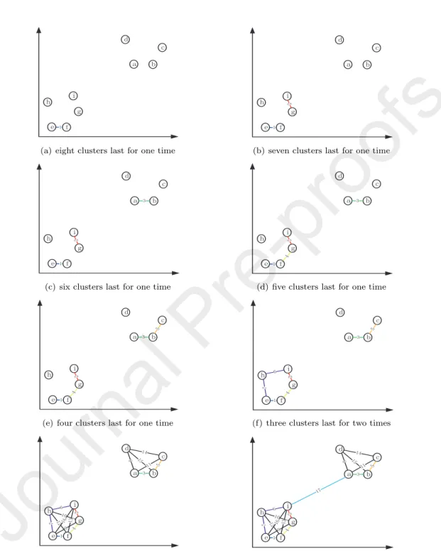
To illustrate the idea of Algorithm 4, we take 9 initial cluster centers as an example to show the merging process in Figure 4.
Fig. 4(a) shows the 9 initial cluster centers. It can be seen that the distance between Points e and f is the shortest. So we merge the two corresponding clusters into one while keeping two cluster centerseandf. And then we obtain
300
eight clusters. The eight clusters last for one time.
In Fig. 4(b), it can be found that the distance between Points g and i is the shortest in the remaining cluster centers. Therefore, we merge the two corresponding clusters into one while keepinggandias the cluster centers, and
D E F G
H I J K
L
(a) eight clusters last for one time
D E
F G
H I J K
L
(b) seven clusters last for one time
D E
F G
H I J K
L
(c) six clusters last for one time
D E
F G
H I J K
L
(d) five clusters last for one time
D E
F G
H I J K
L
(e) four clusters last for one time
D E
F G
H I J K
L
(f) three clusters last for two times
D E
F G
H I J K
L
(g) two clusters last for nine times
D E
F G
H I J K
L
(h) one cluster
Figure 4: Merging process of initial cluster centers
Algorithm 4Merging process (C).
1: Calculate the point-to-point distance of initial cluster centers, and then queue them in ascending order;
2: whilethe number of clusters >1do
3: Sequentially find the two cluster centers which are the nearest currently in the queue;
4: if they are not in the same classthen
5: Merge the two corresponding clusters into one;
6: Count the number of clusters;
7: else
8: Count the number of clusters;
9: end if
10: end while
11: Find the number of clusters which keeps unchanged the most merging times;
12: Find the corresponding clusters;
13: return;
obtain seven clusters. The seven clusters last for one time.
305
In Fig. 4(c), it can be found that the distance between Pointsaandbis the shortest. Therefore, we merge the two clusters with two cluster centers aand b, and obtain six clusters. The six clusters last for one time.
In Fig. 4(d), we can see that Points g and f are the next to be merged.
We merge the two corresponding clusters but still keepg andf as the cluster
310
centers in the merged cluster, and obtain five clusters. The five clusters last for one time.
In Fig. 4(e), we can see that Points bandc are the next to be merged. We merge the two corresponding clusters but still keepbandcas the cluster centers in the merged cluster, and obtain four clusters. The four clusters last for one
315
time.
It can be found in Fig. 4(f) that the distance between Points hand i are the shortest. We merge the two corresponding clusters but still keephandias the cluster centers in the merged cluster, and obtain three clusters. Then, the distance between Pointseandhare the shortest, buteandhare already in one
320
cluster and no merging is needed. Therefore, three clusters last for two times.
In Fig. 4(g), it can be found that Pointsaanddare the next to be merged.
After merging, we obtain two clusters and they last one time. Next, the distance between Points eand g is the shortest, but they have belonged to one cluster
and thus no merging is needed. Therefore, there are still two clusters and they
325
last two times. In the following merging process, the two clusters will last nine times.
It can be found in Fig.4(i) that the distance between Pointsa andi is the next to be merged. After merging, we obtain one cluster, and the merging process is finished.
330
Because the two clusters last for the most merging times (9 times), the final number of clusters is two and the two corresponding clusters are the final clusters. The clustering process ends.
3.5. Time Complexity Analysis of the Proposed Algorithm DPADN
For a data setS={x1,x2,· · ·,xn}, the cost of computing the distance matrix
335
is of orderO(n2). The time to calculate densityρand distanceδis also of order O(n2). The time required to select the initial cluster centers is O(n). If K initial cluster centers are selected (usuallyK ≪n, supposing O(K2log2K)<
O(n2)), the time consumption for sorting K(K-1)/2 distances generated byK initial cluster centers is O(K2log2K). The time complexity of the merging
340
initial cluster centers isO(n). Therefore, the time cost of the proposed DPADN algorithm is stillO(n2).
4. Experiments
We first compare the performance of the density metric function of DPADN with that of FSFDP[34], and then compare the performance of algorithm D-
345
PADN, which automatically determines the clustering center, with that of the algorithm iFSFDP[34], which needs manual selection of clustering centers in two typical data sets. Finally, we compare the performance of the DPADN algorith- m with that of the existing algorithms iFSFDP[34], WOCIL[33], OCIL[42], and RPCCL[32] in ten data sets.
350
4.1. Utilized Data Sets
The ten widely used data sets Flame, Aggregation, Jain, Smiles, Double- circle, Spiral, Iris, Wine, Heart, and Soybean (URL:http://cs.uef.f i/sipu/datasets/
andhttp://archive.ics.uci.edu/ml/) are used in the experiments. These data sets have different numbers of data points and different shapes. Some of them
355
are convex data sets, while others are non-convex ones. The differences between clusters in these data sets are so small that it is difficult to distinguish them.
Table 1 lists the information of all these data sets.
Table 1: The Testing Data Sets
Data set Samples Attributes Clusters
Flame 240 2 2
Aggregation 788 2 7
Jain 373 2 2
Smile 266 2 3
Double-circle 152 2 2
spiral 1000 2 2
Iris 150 4 3
Wine 178 13 3
Heart 303 13 2
Soybean 47 35 4
4.2. Comparison of Density Metrics
The density metric in FSFDP[34] may give the same density value to different
360
points and thus cannot effectively distinguish the densities of points, while the proposed density metric in DPADN will give different density values to different points and thus can distinguish the densities of points. To identify this fact, we compare the density metric in FSFDP[34] with the proposed density metric in DPADN in the experiments. We have demonstrated how many data points
365
correspond to the same density value for each density metric. If more than
one data points correspond to one density value, this means that the density metric used cannot distinguish the densities of different data points effectively.
Otherwise, if each density value corresponds only to one data point, this means that the density metric used can effectively distinguish the densities of different
370
data points.
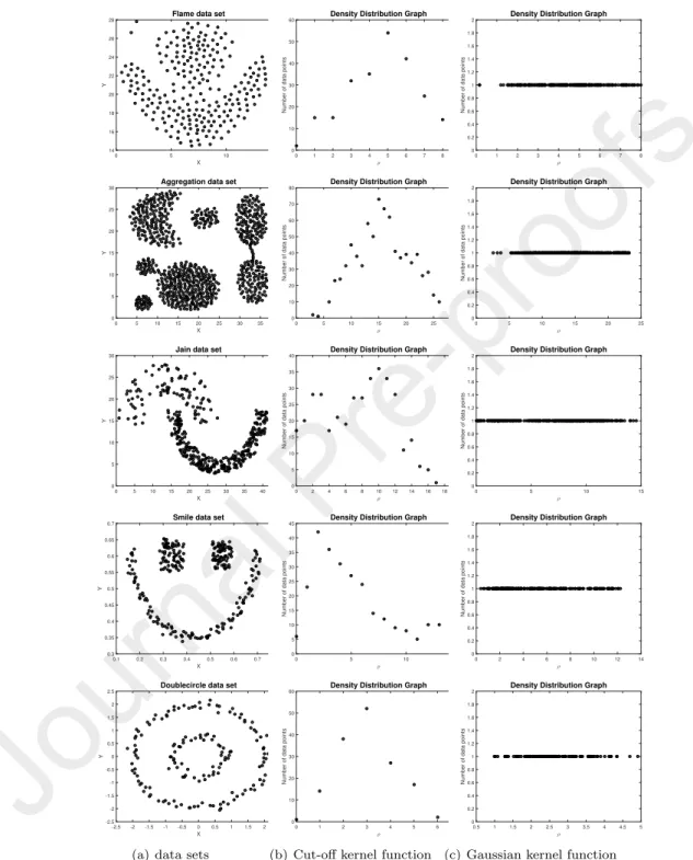
Figure 5 demonstrates the capability of distinguishing the densities of dif- ferent data points by using the Gaussian kernel metric adopted in DPADN and by using the Cut-off kernel metric in FSFDP, where the sub-figures in Column one show the distribution of data sets Flame, Jain, Smiles, Aggregation and
375
Double-circle, respectively. The sub-figures in Columns two and three show the density distribution graph (i.e., the number of data points in the vertical axis vs density value for two density metrics in the horizontal axis) in FSFDP and DPADN, respectively. Sub-figures on each row show these results for one data set.
380
From the sub-figures in Column 2 of Figure 5, we can see clearly that many data points have the same density (corresponding to the density metric in FSFD- P), and from the sub-figures in Column 3, we can see that each density value corresponds to only one data point (corresponding to the density metric in DPADN). This means that the metric used in FSFDP can not effectively dis-
385
tinguish the densities of different data points, while the density metric used in DPADN can.
In addition, the density metric in FSFDP may result in more than one points with the same density ρ and the same distance δ on the decision graph (i.e., more than one points overlap with each other). In this scenario, we do not
390
know how many points will be selected as the cluster centers by using FSFDP [34]. It is very likely to choose a wrong number of cluster centers and thus get wrong clustering results. Also, even if the number of cluster centers is known in advance, we can not know which points overlapped should be chosen as the cluster centers. To illustrate this problem, we calculated the number of the
395
groups of points with the same density and distance in the five data sets Flame, Jain, Smiles, Aggregation and Double-circle, respectively. The results are shown
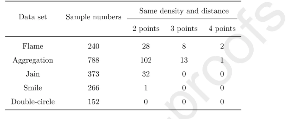
in Table 2.
Table 2: Statistics on the number of groups of points with the same density and distance
Data set Sample numbers Same density and distance 2 points 3 points 4 points
Flame 240 28 8 2
Aggregation 788 102 13 1
Jain 373 32 0 0
Smile 266 1 0 0
Double-circle 152 0 0 0
In Table 2, the number in Column “2 points” represents the number of pairs of points which have the same density and distance, the number in Column “3
400
points” represents the number of groups of 3 points which have the same density and distance, and the number of Column “4 points” is the number of groups of 4 points which have the same density and distance. From Table 2, we can see that there are many pairs or groups of points which have the same density and distance in each data set except for data sets Smile and Double-circle, i.e.,
405
there are many groups in which data points are overlapped in the decision graph in FSFDP, especially for the first three data sets. This means that when we choose these overlapped data points as the cluster centers, we may choose a wrong number of cluster centers. For example, for data set Aggregation, there are 102 pairs of data points overlapped, but each pair appears only as one point
410
in the decision graph. Therefore, for such points, we do not know whether one or two points we should choose as the cluster centers. This may result in choosing a wrong number of cluster centers. Also, even if we know the number of cluster centers and the overlapped points in advance, we cannot determine which data points among the overlapped data points should be selected as the
415
cluster centers in the decision graph by using FSFDP. This may result in a wrong clustering result.
X
0 5 10 15
Y
14 16 18 20 22 24 26
28 Flame data set
X
0 5 10 15 20 25 30 35 40
Y
0 5 10 15 20 25
30 Aggregation data set
X
0 5 10 15 20 25 30 35 40 45
Y
0 5 10 15 20 25
30 Jain data set
X
0.1 0.2 0.3 0.4 0.5 0.6 0.7 0.8
Y
0.3 0.35 0.4 0.45 0.5 0.55 0.6 0.65
0.7 Smile data set
X
-2.5 -2 -1.5 -1 -0.5 0 0.5 1 1.5 2 2.5
Y
-2.5 -2 -1.5 -1 -0.5 0 0.5 1 1.5 2
2.5 Doublecircle data set
(a) data sets
ρ
0 1 2 3 4 5 6 7 8 9
Number of data points
0 10 20 30 40 50
60 Density Distribution Graph
ρ
0 5 10 15 20 25 30
Number of data points
0 10 20 30 40 50 60 70
80 Density Distribution Graph
ρ
0 2 4 6 8 10 12 14 16 18 20
Number of data points
0 5 10 15 20 25 30 35
40 Density Distribution Graph
ρ
0 5 10 15
Number of data points
0 5 10 15 20 25 30 35 40
45 Density Distribution Graph
ρ
0 1 2 3 4 5 6 7
Number of data points
0 10 20 30 40 50
60 Density Distribution Graph
(b) Cut-off kernel function
ρ
0 1 2 3 4 5 6 7 8
Number of data points
0 0.2 0.4 0.6 0.8 1 1.2 1.4 1.6 1.8
2 Density Distribution Graph
ρ
0 5 10 15 20 25
Number of data points
0 0.2 0.4 0.6 0.8 1 1.2 1.4 1.6 1.8
2 Density Distribution Graph
ρ
0 5 10 15
Number of data points
0 0.2 0.4 0.6 0.8 1 1.2 1.4 1.6 1.8
2 Density Distribution Graph
ρ
0 2 4 6 8 10 12 14
Number of data points
0 0.2 0.4 0.6 0.8 1 1.2 1.4 1.6 1.8
2 Density Distribution Graph
ρ
0.5 1 1.5 2 2.5 3 3.5 4 4.5 5
Number of data points
0 0.2 0.4 0.6 0.8 1 1.2 1.4 1.6 1.8
2 Density Distribution Graph
(c) Gaussian kernel function
Figure 5: Density distributions using different density metrics
As discussed above, the density metric used in FSFDP will result in over- lapped points in the decision graph, which may cause two problems: 1) We may select a wrong number of clusters and get wrong cluster results. 2) It is difficult
420
to determine which one/ones of the overlapped points should be selected as clus- ter centers, even if the number of clusters is known in advance. However, the density metric in DPADN (i.e., Gaussian kernel function as the density metric) has no such problems.
4.3. Comparison of DPADN with 4 Existing Algorithms
425
In this section, we will compare DPADN with 4 state-of-the-art algorithms, iFSFDP, WOCIL[33], OCIL[42], and RPCCL[32], in two parts. In the first part, we compare DPADN with an improved FSFDP called iFSFDP to intuitively demonstrate the good performance of DPADN and the difficulty for FSFDP to select a correct number of cluster centers. The iFSFDP is an improved version
430
of FSFDP developed by replacing the original density metric with the Gaussian kernel function. Even so, we shall verify that iFSFDP still does not perform as well as DPADN in the first part of the experiments.
In order to intuitively demonstrate the performance of the compared algo- rithms, we select two widely used two-dimensional data sets so that the clus-
435
tering results obtained can be visually displayed in the figures. The comparison results are shown in Figure 6 and Figure 7.
Figure 6 is the results on data set Aggregation. Fig.6(a) is the decision graph of iFSFDP. Because iFSFDP needs manual selection of cluster centers in the decision graph, we will obtain a correct clustering result if we manually
440
select seven points (correct number) in the red rectangle in Fig.6(a) as the cluster centers, and the result is shown in Fig.6(b). But if we select ten points (incorrect number) in the red rectangle as cluster centers in Fig.6(c), we will obtain a wrong clustering result as shown in Fig.6(d).
Figs. 6(e)-6(h) show the results obtained by using DPADN. DPADN does
445
not need manual selection of the cluster centers. It automatically obtains the initial cluster centers from the decision graph, and then merges the initial cluster
(a)
0 5 10 15 20 25 30 35 40
0 5 10 15 20 25
30 Clustering result
(b) (c) (d)
ρ
0 5 10 15 20 25
δ
0 5 10 15
Decision Graph
(e) (f) (g) (h)
Figure 6: Clustering result on data set Aggregation
(a)
0 5 10 15 20 25 30 35 40 45
0 5 10 15 20 25
30 Clustering result
(b) (c)
0 5 10 15 20 25 30 35 40 45
0 5 10 15 20 25
30 Clustering result
(d)
ρ
0 5 10 15
δ
0 2 4 6 8 10 12
Decision Graph
(e)
ρ
0 5 10 15
δ
0 2 4 6 8 10 12
Merged result in Decision Graph
(f)
0 5 10 15 20 25 30 35 40 45
0 5 10 15 20 25 30
Merged result in raw data set
(g)
0 5 10 15 20 25 30 35 40 45
0 5 10 15 20 25 30
Clustering result
(h)
Figure 7: Clustering result on data set Jain
centers to obtain the final clusters. Fig.6(e) is the decision graph of DPADN, where DPADN automatically selects the data points whose densities are larger than the average density ρ and whose distances are larger than the average
450
distanceδas the initial cluster centers. These initial cluster centers are shown by the points in non-black colors in Fig.6(e). Then, DPADN automatically merges these initial cluster centers and the corresponding clusters into seven bigger clusters. Fig.6(f) shows the merged result of initial cluster centers in the decision graph. The merged cluster centers in the data set, i.e., seven bigger
455
cluster centers, are shown in Fig.6(g). The final seven clusters are shown in Fig.6(h).
Figure 7 shows the results obtained by iFSFDP and DPADN on data set Jain. Figs. 7(a) and 7(c) are the decision graphs of iFSFDP and Figs.7(b) and 7(d) are the corresponding clustering results. Note that even if a correct number
460
of cluster centers are selected as shown in Fig. 7(a), iFSFDP does not give the correct clustering result as shown in Fig.7(b). Of course, it is possible to select a wrong number of cluster centers manually as shown in Fig7(c), which will result in wrong clusters as shown in Fig.7(d). Figs.7(e)-7(h) show the results obtained by DPADN, where Fig.7(e) is the decision graph of DPADN. For this data set,
465
DPADN identifies that there is not any noise point and automatically selects the initial cluster centers shown in Fig.7(e) in non-black colors. Then Fig.7(f) shows the merged result of the initial cluster centers in the decision graph, in which the initial cluster centers are merged into two groups of initial cluster centers.
The points in the same color (blue or green) are in one group. To intuitively
470
demonstrate which real data is the initial cluster centers and which initial cluster centers are merged into one group, we show the merged initial cluster centers in the original data set in Fig.7(g), in which the data points in the same color are in one group. The final clustering results are shown in Fig.7(h). It can be seen from Fig. 7(h) that DPADN obtains correct clusters. The experimental results above
475
indicate that even if FSFDP employs the Gaussian kernel function as the density metric, it is still difficult to select correct cluster centers manually. Even if the number of cluster centers is correctly selected, the clustering result may still
be wrong. However, DPADN does not need any manual operation, and it can automatically identify the noise points and determine the proper initial cluster
480
centers. Furthermore, it can automatically merge the initial cluster centers and the corresponding initial clusters to obtain the correct clustering result.
In the second part of the experiments, we compare DPADN with four algo- rithms: iFSFDP, WOCIL[33], OCIL[42], and RPCCL[32] on 10 data sets. Two popular performance measures, i.e., clustering ACCuracy(ACC), and Rand In-
485
dex(RI), are adopted to evaluate the clustering results. The larger the values of these two measures, the better the performance. The clustering results of all compared algorithms in terms of ACC and RI are presented in Tables 3-4.
In the experiments, for iFSFDP, we always select a true number of clusters (in actual situations, it is hard to do so as discussed in the first part of the
490
experiments) and select the initial numberkof clusters greater than or equal to the true number of clusters for WOCIL, OCIL, and RPCCL. We assign other parameters of these algorithms according to the methods in [34, 33, 42, 32], respectively. From the experimental results, we can see that DPADN performs much better than RPCCL on all data sets, outperforms iFSFDP on 7 data sets
495
and performs as well as iFSFDP on 3 data sets. Also, DPADN performs better than OCIL on 9 data sets and worse than OCIL on the Heart data set. DPADN outperforms WOCIL on 6 data sets and performs worse than WOCIL on 2 data sets Wine and Heart. Note that the Heart data set is a mixed attribute data set (with 13 attributes, 7 categorical attributes and 6 numerical attributes),
500
while WOCIL and OCIL are specifically designed clustering methods for mixed attributed data sets. It is normal for WOCIL and OCIL to outperform DPADN on these data sets. Furthermore, WOCIL is a well designed subspace clustering algorithm and seems to perform better than DPADN on high-dimensional data sets.
505
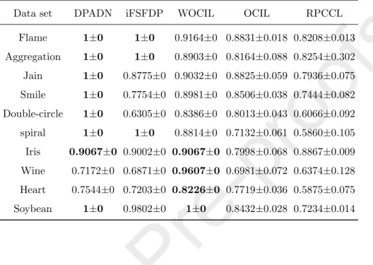
Table 3: Clustering Performances of Different Algorithms in Terms of ACC
Data set DPADN iFSFDP WOCIL OCIL RPCCL
Flame 1±0 1±0 0.9164±0 0.8831±0.018 0.8208±0.013 Aggregation 1±0 1±0 0.8903±0 0.8164±0.088 0.8254±0.302 Jain 1±0 0.8775±0 0.9032±0 0.8825±0.059 0.7936±0.075 Smile 1±0 0.7754±0 0.8981±0 0.8506±0.038 0.7444±0.082 Double-circle 1±0 0.6305±0 0.8386±0 0.8013±0.043 0.6066±0.092 spiral 1±0 1±0 0.8814±0 0.7132±0.061 0.5860±0.105 Iris 0.9067±0 0.9002±0 0.9067±0 0.7998±0.068 0.8867±0.009 Wine 0.7172±0 0.6871±0 0.9607±0 0.6981±0.072 0.6374±0.128 Heart 0.7544±0 0.7203±0 0.8226±0 0.7719±0.036 0.5875±0.075 Soybean 1±0 0.9802±0 1±0 0.8432±0.028 0.7234±0.014
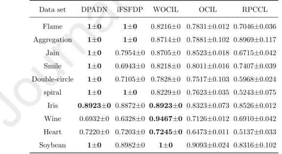
Table 4: Clustering Performances of Different Algorithms in Terms of RI
Data set DPADN iFSFDP WOCIL OCIL RPCCL
Flame 1±0 1±0 0.8216±0 0.7831±0.012 0.7046±0.036 Aggregation 1±0 1±0 0.8714±0 0.7881±0.102 0.8969±0.117 Jain 1±0 0.7954±0 0.8705±0 0.8523±0.018 0.6715±0.042 Smile 1±0 0.6943±0 0.8218±0 0.8011±0.016 0.7407±0.039 Double-circle 1±0 0.7105±0 0.7828±0 0.7517±0.103 0.5968±0.024 spiral 1±0 1±0 0.8229±0 0.7623±0.035 0.5243±0.075 Iris 0.8923±0 0.8872±0 0.8923±0 0.8323±0.073 0.8526±0.012 Wine 0.6932±0 0.6328±0 0.9467±0 0.7126±0.012 0.6910±0.042 Heart 0.7220±0 0.7203±0 0.7245±0 0.6473±0.011 0.5137±0.033 Soybean 1±0 0.8982±0 1±0 0.9093±0.024 0.8316±0.102
5. Conclusion
In this paper, we propose a new clustering algorithm called DPADN which includes the following new schemes: 1) A new density metric (Gaussian kernel function as the density metric), which can avoid points overlapping in the de- cision graph. 2) An effective algorithm to determine the initial cluster centers
510
automatically. 3) A merging scheme for the initial cluster centers and the cor- responding clusters. DPADN is fully automatic and does not need any manual operation or any parameter input. It can be concluded from the experiments that DPADN outperforms iFSFDP and RPCCL completely and performs better than OCIL and WOCIL on most test data sets. It seems that DPADN does
515
not perform as well as WOCIL on mixed attribute data and high dimensional data. In the future, it is necessary to add some new schemes into DPADN to deal with mixed attribute data and high dimensional data.
Acknowledgment
This work was supported by the National Natural Science Foundation of
520
China (No.61872281), and by National Key Research and Development Program of China (2017YFC1703506).
References
[1] R. Michalski, I. Bratko, M. Kubat, Machine Learning and Data Mining:
Methods and Applications, Wiley, 1998.
525
[2] G. Wang, Q. Song, Automatic clustering via outward statistical testing on density metrics, IEEE Transactions on Knowledge and Data Engineering 28 (8) (2016) 1971–1985.
[3] J. L. Bruse, M. A. Zuluaga, A. Khushnood, K. McLeod, H. N. Ntsinjana, T.-Y. Hsia, M. Sermesant, X. Pennec, A. M. Taylor, S. Schievano, Detecting
530
clinically meaningful shape clusters in medical image data: Metrics analysis
for hierarchical clustering applied to healthy and pathological aortic arches, IEEE Transactions on Biomedical Engineering 64 (10) (2017) 2373–2383.
[4] W. C. Liew, H. Yan, M. Yang, Pattern recognition techniques for the emerg- ing field of bioinformatics: a review, Pattern Recognition 38 (11) (2005)
535
2055–2073.
[5] J. Gao, M. T. Chang, H. C. Johnsen, S. P. Gao, B. E. Sylvester, S. O.
Sumer, H. Zhang, D. B. Solit, B. S. Taylor, N. Schultz, 3D clusters of somatic mutations in cancer reveal numerous rare mutations as functional targets, Genome Medicine 9 (1) (2017) 4.
540
[6] C.-C. Chen, X. Fu, C.-Y. Chang, A terms mining and clustering technique for surveying network and content analysis of academic groups exploration, Cluster Computing 20 (1) (2017) 43–52.
[7] Y. Li, C. Luo, S. M. Chung, Text clustering with feature selection by using statistical data, IEEE Transactions on Knowledge and Data Engineering
545
20 (5) (2008) 641–652.
[8] D. Fu, S. He, New combination algorithms in commercial area data min- ing and clustering, in: 2016 IEEE International Conference on Big Data Analysis (ICBDA), IEEE, 2016, pp. 1–5.
[9] S. L. Hao, The customer segmentation of commercial banks based on u-
550
nascertained clustering, in: International Conference on Logistics Systems and Intelligent Management, 2010, pp. 297–300.
[10] C. Cooper, D. Franklin, M. Ros, F. Safaei, M. Abolhasan, A comparative survey of vanet clustering techniques, IEEE Communications Surveys and Tutorials 19 (1) (2017) 657–681.
555
[11] Y. Li, L. Li, D. Li, F. Yang, Y. L. Liu, A density-based clustering method for urban scene mobile laser scanning data segmentation, Remote Sensing 9 (4) (2017) 331–349.
[12] X. Duan, Y. Liu, X. Wang, SDN enabled 5G-VANET: Adaptive vehicle clustering and beamformed transmission for aggregated traffic, IEEE Com-
560
munications Magazine 55 (7) (2017) 120–127.
[13] Lenc, Ladislav, Kral, Pavel, Local binary pattern based face recognition with automatically detected fiducial points, Integrated Computer Aided Engineering 23 (2) (2016) 129–139.
[14] M. Wozniak, D. Polap, Object detection and recognition via clustered fea-
565
tures, Neurocomputing 320 (2018) 76–84.
[15] L. T. Law, Y. M. Cheung, Color image segmentation using rival penalized controlled competitive learning, in: Neural Networks, 2003. Proceedings of the International Joint Conference on, 2003.
[16] M. S. Pera, Y. K. Ng, Utilizing phrase-similarity measures for detecting
570
and clustering informative rSS news articles, Integrated Computer Aided Engineering 15 (4) (2010) 331–350.
[17] J. W. Wu, J. C. R. Tseng, W. N. Tsai, A hybrid linear text segmentation algorithm using hierarchical agglomerative clustering and discrete particle swarm optimization, Integrated Computer Aided Engineering 21 (1) (2014)
575
35–46.
[18] M. Wang, W. Zuo, W. Ying, An improved density peaks-based clustering method for social circle discovery in social networks, Neurocomputing 179 (2016) 219–227.
[19] Amit, Saxena, Mukesh, Prasad, Akshansh, Gupta, Neha, Bharill, Om,
580
Prakash, A review of clustering techniques and developments, Neurocom- puting 267 (2017) 664–681.
[20] G. M. Mazzeo, E. Masciari, C. Zaniolo, A fast and accurate algorithm for unsupervised clustering around centroids, Information Sciences 400 (2017) 63–90.
585
[21] A. Fahad, N. Alshatri, Z. Tari, A. Alamri, A. Bouras, A survey of clus- tering algorithms for big data: Taxonomy and empirical analysis, IEEE Transactions on Emerging Topics in Computing 2 (3) (2014) 267–279.
[22] J. MacQueen, Some methods for classification and analysis of multivariate observations, in: Proceedings of the 5th Berkeley Symposium on Mathe-
590
matical Statistics and Probability, 1967, pp. 281–297.
[23] J. Huang, M. Ng, H. Rong, Z. Li, Automated variable weighting in k-means type clustering, IEEE Transactions on Pattern Analysis and Machine In- telligence 27 (5) (2005) 657–668.
[24] L. Jing, M. K. Ng, J. Z. Huang, An entropy weighting k-means algorithm
595
for subspace clustering of high-dimensional sparse data, IEEE Transactions on Knowledge and Data Engineering 19 (8) (2007) 1026–1041.
[25] Z. Tian, R. Ramakrishnan, M. Livny, BIRCH: an efficient data clustering method for very large databases, in: ACM SIGMOD International Confer- ence on Management of Data, 1996, pp. 103–114.
600
[26] Z. Tian, R. Ramakrishnan, M. Livny, BIRCH: a new data clustering al- gorithm and its applications, Data Mining and Knowledge Discovery 1 (2) (1997) 141–182.
[27] M. Ester, H.-p. Kriegel, J. Sander, X. Xu, A density-based algorithm for discovering clusters in large spatial databases with noise, in: International
605
Conference on Knowledge Discovery and Data Mining, 1996, pp. 226–231.
[28] A. C. Bryant, K. J. Cios, RNN-DBSCAN: a density-based clustering algo- rithm using reverse nearest neighbor density estimates, IEEE Transactions on Knowledge and Data Engineering 30 (6) (2018) 1109–1121.
[29] W. Wang, J. Yang, R. R. Muntz, STING: a statistical information grid
610
approach to spatial data mining, in: Vldb’97, Proceedings of International Conference on Very Large Data Bases, 1997, pp. 186–195.