For the trained models, the effectiveness of the bone removal algorithm and windowing was investigated. Furthermore, this thesis investigates the effects of the bone removal algorithm, window magnifications, model performance and channel sensitivity.
Articular cartilage: composition structure and function 12
Articular cartilage supports a large part of the joint pressure by integrating the synovial fluid, which is incompressible. The extracellular matrix of articular cartilage possesses unique mechanical properties such as viscoelasticity and poroelasticity which in return contribute to the bulk mechanical properties of the tissue.
Articular cartilage degeneration and characterization 13
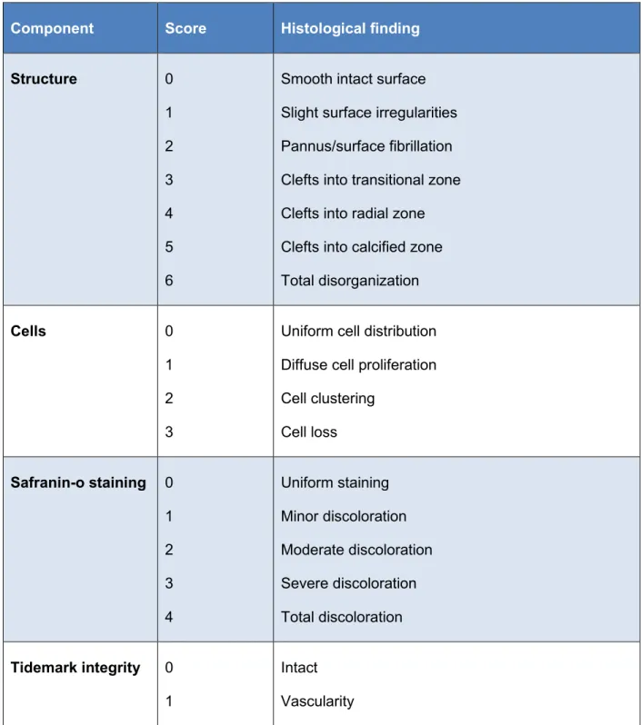
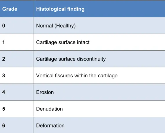
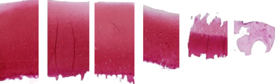
One of the other features associated with articular cartilage degeneration is the detachment of the collagen network. One of the most commonly used systems for this purpose is the one proposed by Mankin [3].
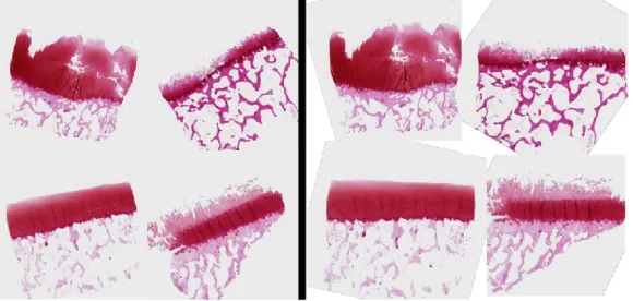
![Figure 2.1: Comparing OA with a normal tissue [18].](https://thumb-eu.123doks.com/thumbv2/9pdfco/1891408.267574/15.918.462.805.299.611/figure-comparing-oa-with-a-normal-tissue.webp)
Mankin scoring 16
Components of Mankin scoring 16
Smooth, intact surface Slight surface irregularities Pannus/surface fibrillation Fissures in the transitional zone Fissures in the radial zone Fissures in the calcified zone Total disorganization.
OARSI scoring 18
This means that the data in the presented matrix can be used to classify parts of the image or the entire image into the desired categories. This approach assumes that part of the source domain labeled data can be reused for the target domain after reweighting or resampling. Generative models can be used to transfer knowledge about learned features [70, 71].
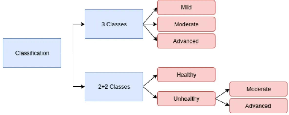
The algorithm is based on the color, texture, color saturation and relative location of the elements. The impact of this algorithm on the performance of the models is explored and reported in the results and discussion sections. The three-class classification approach labeled images as one of three classes of "mild".
This may be due to the increased number of possible outputs (before and without applying the softmax layer). This may suggest the importance of the initial layers of the network covering the basic generic functions.
Limitations of the histopathological scoring systems 19
Single-layer perceptron 24
A single-layer perceptron is a simple single-layer neural network in which the output is defined as the linear combination of the input variables plus a bias term. The bias, b, is scalar, while the input x and the weights w are vectors, that is, x ∈ ℝn and w ∈ ℝn with n ∈ ℕ, representing the dimension of the input.
Supervised learning algorithm for a perceptron 25
Multi-layer perceptron 25
Backpropagation 26
Batch size, iterations, and epochs 26
Overfitting 27
Machine learning and deep learning 27
Artificial neural networks are machine learning methods that can be used in both supervised and unsupervised approaches. Shallow neural networks contain few hidden layers, while deep neural networks contain many hidden layers.
Computer vision and neural networks 27
In reinforcement learning, a “policy network” is used to “reward” or “punish” an agent (acting on an input data set) for each individual input without using pre-labeled goals. Some of the traditional algorithms in machine learning include decision trees, Bayesian networks, support vector machines (SVM), etc.
Convolutional neural networks 28
- Convolutional layer 28
- Fully connected layer 29
- Activation layer 29
- Pooling layer 29
- Dropout 29
This layer is similar to a simple neural network layer where each node is connected to all nodes in the previous layer. This layer is usually inserted between 2 or 3 convolution layers and reduces the parameter requirement.
Popular CNN model architectures 29
AlexNet 30
VGG 30
ResNet 31
Machine learning for automated histopathological grading 32
Technical features provide more transparency and will then generally appear more instinctive to the end user – the pathologist or physician, as the case may be. However, the uncontrolled feature generation approach of deep learning strategies can be quickly and seamlessly applied to any domain or problem, but suffers from the lack of feature interpretability [57].
Transfer learning 33
- Theory and background 33
- Definition 34
- Transfer learning types 35
- Instance-based transfer learning 35
- Feature-based transfer learning 36
- Model-based transfer learning 37
- Relation-based transfer learning 39
- Adversarial transfer learning 39
- Similar studies 40
Knowing this inequality, transfer learning can be defined as any use of the knowledge in Ds and Ts to improve the predictive function in the target domain ft. The idea behind feature-based approaches is to identify a good feature representation for both domains, so that by projecting data onto the new representation, the source domains called data can be reused for training in the target domain [58,60]. Thus, for a related task in the target domain, this structure can be transferred to train an accurate target model 𝜃𝑡 with labeled data in the target domain.
When using deep learning models, parameters from a pre-trained deep learning model can be used to initialize the target domain model(s).
Histopathological grading 43
Sample collection 43
Histology assessment 43
Histology scoring 43
Preprocessing 44
Rotation 44
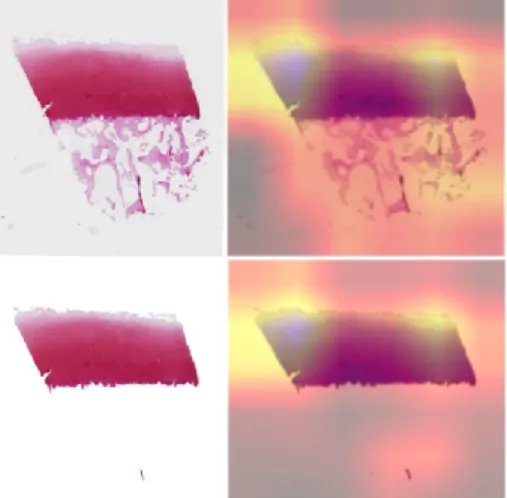
Figure 7.6 shows the activations of the middle layer of the AlexNet-based model developed for the classification problem. This emphasizes the importance of dropouts, perhaps reducing the effect of white areas. If these two abnormal sets (set 8 and 9) are not used, the accuracy is the best 2+2-classification.
When bone sweep is not used, calcified fragments are the main cause of error (Figure 8.5).
Bone deletion 45
Augmentation and Windowing 46
Augmentation typically consists of adding rotated and flipped copies of the original images to the training dataset. Different magnification sizes were tested using cross-validation, the tenfold size was found to avoid overfitting and showed the best results. The width of each window is set to be one third of the input image (wl = width/3).
Using cross-validation of all input images, the best value of n was found to be 4.
Deep learning-based scoring 46
Dataset 47
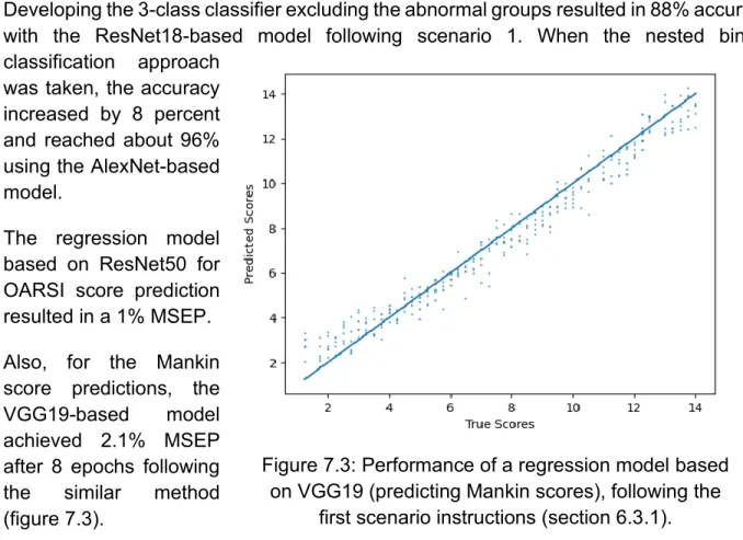
Images from corpses 8 and 9 were recorded using a different camera setting, thus clearly showing different low-level image features (eg, contrast and color). These images were labeled by the Mankin and OARSI scoring systems and all possible scores were observed in the dataset. Regression models were developed to predict a real number value in the range of these scoring systems (0-14 for Mankin, 0-6 for OARSI).
The classification model was developed to assess tissue integrity in three different classes based on specific thresholds applied to the Mankin score (mild: score<4, moderate: .4
Learning procedure 48
The softmax layer finally uses the softmax function, also known as softargmax or normalized exponential function, which is a generalization of logistic. The output layer of the models includes a softmax activation function to map the output of the network to a probability distribution over the target classes. The softmax function takes as input a vector of real numbers and normalizes it into a probability distribution consisting of K (number of classes) probabilities proportional to the exponents of the input numbers.
Before this function is applied, the vector of numbers is not limited to any class and is distributed within a certain linear range, at this point (before the softmax layer), this vector can be extracted to be considered as a regression output.
Model performance analysis 50
Classification 50
Before applying the softmax layer, some vector components may be negative or greater than 1, but after applying softmax, the components will be normalized to the interval of [0, 1] with their sum equal to 1, so they can be interpreted as probabilities. Since the classification is nested, the accuracy of moderate/advanced (second part) is reported multiplied by the accuracy of healthy/unhealthy classification.
Regression 51
CAMs and visualization of activations 51
Class activation maps 51
Using a concept called global average pooling, one study [91] successfully used the advantages of this global average pooling layer for localization capability to the last layer.
Visualization of activation layers 52
Standard deviation of difference 52
Model deployment 52
This method is called class activation mapping and it points to the most important regions leading to a specific network output (eg a class). Limitations on the file upload and used libraries had to be introduced directly to the serving host. Necessary codes and files were pushed to a GitHub page and deployed to the server (figure 6.6).
The client is provided with basic image processing and data analysis tools such as image resizing and data preprocessing.

Preprocessing 54
Excluding the abnormal groups 55
Including the abnormal groups 55
Classification 55
Regression 56
Preprocessing effectiveness 58
Visualization of activations and CAMs 58
In addition, to assess the reliability of the AI-driven models, the results of these models in the test set were also compared with the true values (Figure 7.12). This also implies that the depth and complexity of the architecture would not necessarily increase accuracy. In 100% of the samples from the abnormal groups, the green and blue peak channels were indistinguishable.
Interobserver ratings of received scores from human scorers show very poor agreement between them. Proceedings of the 2004 ACM SIGKDD International Conference on Knowledge Discovery and Data Mining - KDD ’04, p. In Proceedings of the 27th International Conference on Neural Information Processing Systems, 2 (NIPS Semi-Supervised Learning Literature Survey, Tech.
Inter-observer variability and comparison with developed models 60
Learning process 64
The training data for this thesis work was not as large as that of popular, well-built and pre-trained CNNs. In addition, some of the necessary filters, features and parameters can be found in most of the early layers of these pre-trained models. Consequently, it was justified to use these pre-trained, tested and high-performing neural networks to take advantage of the already learned parameters and build many of the achieved weights and new parameters on the latter layers and refine the weights with our own. training set (target domain).
Model performance evaluation 64
Model comparison 65
Bone-deletion algorithm effectiveness 65
Impact of windowing on model performance 66
Including the abnormal sets 67
Model losses 68
To note the effect of this difference, 50 random images were selected to compare the color value histograms from each group. Many of the prediction failures are shown to be caused by the model searching through the white areas; although other works have used and shown the effectiveness of replacing pixels with white pixels [101], it is shown here that it can also have its downsides. Also, another misleading feature of this method is the missing calcified parts from the bone sweep algorithm.
Previous works 69
The aim of the thesis was to address the limitations existing in current scoring systems and methods, caused by human error and inefficiencies. With proper pre-processing, the results show that the developed models in this thesis outperform two of the similar works previously proposed for automating the scoring by Mousavi-Harami et al. Collagens: major component of the physiological cartilage matrix, major target of cartilage degeneration, important aid in cartilage repair.
From classical to deep learning: review of cartilage and bone segmentation techniques in knee osteoarthritis research.
87
I.1 AlexNet-based model analysis in 2+2 classification 87
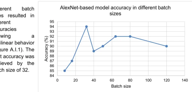
I.1.1 The effect of batch size 87
I.1.2 The effect of epochs 87
I.1.3 The effect of learning rate 88
I.2 ResNet50-based model analysis in Regression (Mankin) 89
I.2.1 The effect of batch size 89
I.2.2 The effect of epochs 89
I.2.3 Visualization of activations 90
I.3 ResNet50-based model analysis in Regression (OARSI) 90
I.3.1 The effect of batch size 90
I.3.2 The effect of epochs 91


![Figure 4.4: VGG architecture [54].](https://thumb-eu.123doks.com/thumbv2/9pdfco/1891408.267574/30.918.201.718.720.1013/figure-vgg-architecture.webp)