Deep Generative Variational Autoencoding for Replay Spoof Detection in Automatic Speaker Verification
Bhusan Chettri, Tomi Kinnunen, Emmanouil Benetos
PII: S0885-2308(20)30025-5
DOI:
https://doi.org/10.1016/j.csl.2020.101092Reference: YCSLA 101092
To appear in:
Computer Speech & LanguageReceived date: 11 November 2019
Revised date: 7 February 2020 Accepted date: 2 March 2020
Please cite this article as: Bhusan Chettri, Tomi Kinnunen, Emmanouil Benetos, Deep Generative Vari- ational Autoencoding for Replay Spoof Detection in Automatic Speaker Verification,
Computer Speech& Language
(2020), doi:
https://doi.org/10.1016/j.csl.2020.101092This is a PDF file of an article that has undergone enhancements after acceptance, such as the addition of a cover page and metadata, and formatting for readability, but it is not yet the definitive version of record. This version will undergo additional copyediting, typesetting and review before it is published in its final form, but we are providing this version to give early visibility of the article. Please note that, during the production process, errors may be discovered which could affect the content, and all legal disclaimers that apply to the journal pertain.
©
2020 Published by Elsevier Ltd.
Highlights
• Variational autoencoder (VAE) for replay spoofing attack detection as an alternative backend to GMMs.
• A systematic comparison of three alternative class-conditioned VAE vari- ants.
• Experimental evaluation on two standard replay spoofing benchmarks, ASVspoof 2017 v2.0 and ASVspoof 2019 PA.
• VAE residual (absolute difference of input and its reconstruction) as a data-driven feature representation for replay attack detection.
Deep Generative Variational Autoencoding for Replay Spoof Detection in Automatic Speaker Verification
Bhusan Chettri1,2, Tomi Kinnunen1, Emmanouil Benetos2
1School of Computing, University of Eastern Finland, FI-80101, Joensuu, Finland
2School of EECS, Queen Mary University of London, United Kingdom
Abstract
Automatic speaker verification(ASV) systems are highly vulnerable to presenta- tion attacks, also called spoofing attacks. Replay is among the simplest attacks to mount — yet difficult to detect reliably. The generalization failure of spoofing countermeasures (CMs) has driven the community to study various alternative deep learning CMs. The majority of them aresupervisedapproaches that learn a human-spoof discriminator. In this paper, we advocate a different,deep gen- erativeapproach that leverages from powerfulunsupervisedmanifold learning in classification. The potential benefits include the possibility to sample new data, and to obtain insights to the latent features of genuine and spoofed speech. To this end, we propose to usevariational autoencoders (VAEs) as an alternative backend for replay attack detection, via three alternative models that differ in their class-conditioning. The first one, similar to the use of Gaussian mixture models (GMMs) in spoof detection, is to train independently two VAEs — one for each class. The second one is to train a single conditional model (C-VAE) by injecting a one-hot class label vector to the encoder and decoder networks. Our final proposal integrates anauxiliary classifierto guide the learning of the latent space. Our experimental results using constant-Q cepstral coefficient (CQCC) features on the ASVspoof 2017 and 2019 physical access subtask datasets indi- cate that the C-VAE offers substantial improvement in comparison to training two separate VAEs for each class. On the 2019 dataset, the C-VAE outper- forms the VAE and the baseline GMM by an absolute 9 - 10% in both equal error rate (EER) and tandem detection cost function (t-DCF) metrics. Finally, we propose VAE residuals — the absolute difference of the original input and the reconstruction as features for spoofing detection. The proposed frontend ap- proach augmented with a convolutional neural network classifier demonstrated substantial improvement over the VAE backend use case.
Keywords: anti-spoofing, presentation attack detection, replay attack, countermeasures, deep generative models.
1. Introduction
Voice biometric systems use automatic speaker verification (ASV) [1] tech- nologies for user authentication. Even if it is among the most convenient means of biometric authentication, the robustness and security of ASV in the face of spoofing attacks (orpresentation attacks) is of growing concern, and is now well acknowledged by the community [2]. A spoofing attack involves illegitimate access to personal data of a targeted user.
The ISO/IEC 30107-1 standard [3] identifies nine different points a biometric system could be attacked from (see Fig. 1 in [3]). The first two attack points are of specific interest as they are particularly vulnerable in terms of enabling an adversary to inject spoofed biometric data. These involve: 1) presentation attack at the sensor (microphone in case of ASV); and 2) modifying biometric samples to bypass the sensor. These two modes of attack are respectively known asphysical access (PA) and logical access (LA) attacks in the context of ASV.
Artificial speech generated throughtext-to-speech(TTS) [4] and modified speech generated throughvoice conversion (VC) [5] can be used to trigger LA attacks.
Playing back pre-recorded speech samples (replay[6]) andimpersonation[7] are, in turn, examples of PA spoofing attacks. Therefore, spoofing countermeasures are of paramount interest to protect ASV systems from such attacks. In this study, acountermeasure (CM) is understood as a binary classifier designed to discriminate real human speech or bonafide samples from spoofed ones in a speaker-independent setting.
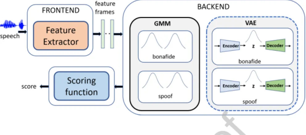
Like any traditional machine learning classifier, a spoofing countermeasure (Fig.1) typically consists of a frontend and a backend module. The key function of the front-end is to transform the raw acoustic waveform to a sequence ofshort- term feature vectors. These short-term feature vectors are then used to derive either intermediate recording-level features (such asi-vectors [8,9] orx-vectors [10]) or statistical models, such as Gaussian mixture models (GMMs) [11] to be used for bonafide or spoof class modeling. In contrast to these approaches that require a certain level of handcrafting especially in the frontend, modern deep-learning based countermeasures are often trained using either raw-audio waveforms [12, 13] or an intermediate high-dimensional time-frequency repre- sentation — often the power spectrogram [14, 15]. In these approaches, the notions of frontend and backend are less clearly distinguished.
In classic automatic speech recognition (ASR) systems and many other speech applications, prior knowledge of speech acoustics and speech percep- tion has guided the design of some successful feature extraction techniques,mel frequency cepstral coefficients (MFCCs) [16] being a representative example.
Similara priori characterization of acoustic cues that are relevant for spoofing attack detection, however, is challenging; this is because many attacks areun- seen, and since the human auditory system has its limits — it is not designed to detect spoofed speech and may therefore be a poor guide in feature crafting.
This motivates the study of data-driven approaches that learn automatically the relevant representations for spoofing detection. In this study, we primarily focus on deep learning based CMs.
Figure 1: An automatic spoofing detection pipeline using a generative model backend. We explore VAEs as an alternative to a GMM backend. In either case, two generative models are trained to learn the distribution of the bonafide and spoof class data. During inference, for a given test utterance, the scoring function computes the log-likelihood difference between the two generative models as a score. See Section3for details on the methodology.
Both discriminative models (such assupport vector machines (SVMs),deep neural networks (DNNs) [17,14]) and generative models (such as GMMs) [11, 15], have extensively been used as backends for spoofing detection. The former directly optimize the class decision boundary while the latter model the data generation process within each of the classes, with the decision boundary being implied indirectly. Both approaches can be used for classification but only the generative approach can be used to sample new data points. We focus on generative modeling as it allows to interpret the generated samples to gain insights about our modeling problem, or to “debug” the deep learning models and illustrate what the model has learned from the data to make decisions.
Further, they can be used for data augmentation which is challenging using purely discriminative approaches.
GMMs have empirically been demonstrated to be competitive in both the ASVspoof 2015 and ASVspoof 2017 challenges [11, 15]. While [11] use hand- crafted features for synthetic speech detection, [15] used deep features to train GMM backends. A known problem with GMMs, however, is that use of high- dimensional (short-term) features often leads to numerical problems due to sin- gular covariance matrices. Even if off-the-shelf dimensionality reduction meth- ods such as principal component analysis (PCA) [18] or linear discriminant analysis (LDA) [19] prior to GMM modeling may help, they are not jointly op- timized with the GMM. Is there an alternative way to learn a generative model that can handle high-dimensional inputs natively?
Three generative models that have been demonstrated to produce excellent results in different applications includegenerative adversarial networks(GANs) [20], variational autoencoders (VAEs) [21] and autoregressive models (for ex- ample, WaveNet [22]). A VAE is a deep generative probabilistic model that consists of anencoder and adecoder network. The encoder (inference network)
transforms the input dataxinto a low-dimensionallatentrepresentation,z, by learning a conditional probability distributionqφ(z|x). The decoder (or genera- tor) network, on the other hand, learns to reconstruct the original data from the low-dimensional latent vector z by learning the conditional probability distri- butionpθ(x|z). GANs, on the other hand, do not have an encoder/recognition network. Instead, they consist of a generator and a discriminator network. The generator takes as input a random vector and aims to generate fake data that is as close to the real datax, and the discriminator network aim is to discriminate between the real and the fake data. Autoregressive models, on the other hand, do not use any latent variables.
Both GANs and VAEs have demonstrated promising results in computer vision [23,24,25], video generation [26] and natural language processing tasks [27]. VAEs have recently been studied for modeling and generation of speech signals [28,29,30], and synthesizing music sounds in [31]. They have also been used for speech enhancement [32, 33] and feature learning for ASR [34, 35].
Recent studies in ASV have studied the use of VAEs indata augmentation[36], regularisation [37] and domain adaptation [38] for deep speaker embeddings (x-vectors). In TTS, VAEs have been recently used to learn speaking style in an end-to-end setting [39]. Recent work in [40] uses VAEs for extracting low-dimensional features and trains a separate classifier on these features for spoofing detection. However, as far as the authors are aware, the application of VAEs as a backend classifier for spoofing attack detection in ASV remains an unexplored avenue.
In this work, we focus on deep probabilistic VAEs as a backend for spoofing detection. Figure1 illustrates our idea. While VAEs have both inference and generator networks, GANs do not have an inference network and autoregressive models do not use latent variables. This motivates our focus on VAEs over other deep generative models, as it suits more naturally our task. The reconstruction quality of VAEs tends to be inferior to that obtained by GANs [41], but for classification tasks, obtaining a perfect reconstruction isnot the main priority.
A key challenge, instead, is how to train VAEs to not only preserve reasonable reconstruction but to allow to retain discriminative information in the latent space. To address this, VAEs are often trained with additional constraints. For example, by conditioning the encoder and decoder with additional input — so called conditional VAE (C-VAE) [42]; or by augmenting anauxiliary classifier either to the latent space [43] or to the output of the decoder network [44]. As there is no de facto standard on this, we aim to fill this knowledge gap in the domain of audio replay detection. In specific, we present a feasibility study of various alternative VAEs for replay spoofing attack detection. We summarize the contributions of this work as follows:
• While deep generative models, VAEs in particular, have been studied in many other domains, their application in audio spoofing detection remains less explored to date. We study the potential of deep generative VAEs as a backend classifier for spoofing detection. To the best of our knowledge, this is the first work in this direction.
• We describe practical challenges in training a VAE model for spoofing de- tection applications and discuss approaches that can help overcome them, which could serve as potential guidelines for others.
• Along with a “naive”1VAE we also study conditional VAEs (C-VAEs) [42].
The C-VAE uses class labels as an additional conditional input during training and inference. Since we pass class labels in C-VAE, we use a single model to represent both classes unlike naive VAE where we train two separate models, one each for bonafide and spoof class. For the text- dependent setting of ASVspoof 2017 data, we further address conditioning using a combination of the class and passphrase labels.
• Inspired by [43, 44], we introduce an auxiliary classifier into our VAE modeling framework and study how this helps the latent space2to capture discriminative information without sacrificing much during reconstruction.
We experiment adding the classifier model on top of the latent space and at the end of the decoder (Section3.3).
• While our primary focus is in using VAEs as a back-end, we also address their potential in feature extraction. In particular, we subtract a VAE- modeled spectrogram from the original spectrogram so as to de-emphasize the importance of salient speech features (hypothesized to be less relevant in spoofing attack detection) and focus on the residual details. We train a convolutive neural network classifier using these residual features.
2. Related work
Traditional methods. Since the release of benchmark anti-spoofing datasets [63,64,65] and evaluation protocols as part of the ongoing ASVspoof challenge series3, there has been considerable research on presentation attack detection [2], in particular for TTS, VC, and replay attacks. Many anti-spoofing features coupled with a GMM backend have been studied and proposed in the litera- ture. We briefly discuss them here. Constant Q cepstral coefficients (CQCCs) [66], among them, have shown state-of-the-art performance on TTS and VC spoofed speech detection tasks on the ASVspoof 2015 dataset [63]. They have been adapted as baseline features in the recent ASVspoof 2017 and ASVspoof 2019 challenges. Further tweaks on CQCCs have been studied in [67] showing some improvement over the standard CQCCs. Teager energy operator (TEO) based spoof detection features have been studied in [68]. Speech demodula- tion features using the TEO and the Hilbert transform have been studied in
1We usenaive VAE to refer the standard (vanilla) VAE [21] trained without any class labels. Information about the class is included by independently training one VAE per class.
2A latent space is a probability distribution that defines the observed-data generation process and is characterised by means and variances of the encoder network.
3http://www.asvspoof.org/
Table1:Summaryofdeeplearningarchitectures/methodsstudiedinthecontextofspoofingdetectioninASV.Disc:discriminative,Gen:generative. D1:ASVspoof2015,D2:BTAS2016,D3.1:ASVspoof2017v1.0,D3.2:ASVspoof2017v2.0,D4:ASVspoof2019LA,D5:ASVspoof2019PA. Metricsreportedareequalerrorrate,EER,andtandemdetectioncostfunction,t-DCF,unlessotherwisestated.Reportednumbersareforthe respectiveevaluationsets. ModelingModel/InputPurposeMetricDatasetF approachArchitecturefeatures[EER/t-DCF]used DiscCNNraw-waveformend-to-end0.157D1 DiscCNN+LSTMraw-waveformend-to-end0.82HTERD2 DiscCNNspectrogramclassification10.6D3.2 DiscLCNN[46]spectrogramembeddinglearning-D3.1 GenGMMsembeddingclassification7.37D3.1 DiscCNNCQCC+HFCCembeddinglearning11.5D3.1feature DiscDNN+RNNFBanks,MFCCsembeddinglearning-D1 DiscSVM,LDAembeddingclassification1.1D1 DiscCNNembeddinglearning-D3.1 GenGMMembeddingclassification6.4D3.1 DiscBayesianDNN,LCNNspectrogramclassification[0.88/0.0219]D5 DiscVGG,SincNet,LCNNspectrogram,CQTclassification[1.51/0.0372]D5 [8.01/0.2080]D4 DiscLCNN,RNNspectrogramembeddinglearning-- GenPLDAembeddingclassification6.08D3.1 DiscLDAembeddingclassification[6.28/0.1523]D4 GenPLDAembeddingclassification[2.23/0.0614]D5 DiscTDNN,LCNN,ResNetCQCCs,LFCCsembeddinglearning[9.08/0.1791]D4 DiscResNet[53]STFT,groupdelaygramclassification[0.66/0.0168]D5 DiscTDNNMFCC,CQCC,spectrogrammultitasking,classification7.94D3.2 [7.63/0.2129]D4 [0.96/0.0266]D5 DiscResNetMFCCs,CQCCsclassification13.30D3.1 DiscResNet,SeNetCQCC,spectrogramclassification[0.59/0.016]D5 [6.7/0.155]D4 DiscResNetMFCCs,CQCC,spectrogramclassification[6.02/0.1569]D4 [2.78/0.0693]D5 DiscCNN+GRUspectrogramclassification[2.45/0.0570]D5 ResNet,LSTMsspectrogramembeddinglearning16.39D3.1 GenGMMsCQCC,LFCC,MelRPclassification11.43D3.2 GenAttention-basedResNetspectrogramclassification8.54D3.2 GenVAECQTspectrogramembeddinglearning-D4 GenVAECQCC,spectrogramclassification,featureextractionD3.2,D5
[69]. Authors in [70] proposed features for spoofing detection by exploiting the long-term temporal envelopes of the subband signal. Spectral centroid based frequency modulation features have been proposed in [71]. [72] proposes the use of decision level feature switching between mel and linear filterbank slope based features, demonstrating promising performance on the ASVspoof 2017 v2.0 dataset. Adaptive filterbank based features for spoofing detection have been proposed in [73]. Finally, [74] proposes the use of convolutionalrestricted Boltzmann machines (RBMs) to learn temporal modulation features for spoof- ing detection.
Deep learning methods. Deep learning-based systems have been pro- posed either for feature learning [47, 15, 17, 48] or in an end-to-end setting to model raw audio waveforms directly [13, 12]. A number of studies [55, 52]
have also focused on multi-task learning for improved generalization by simul- taneously learning an auxiliary task. Transfer learning anddata augmentation approaches have been addressed in [52,54]. Some of the well known deep archi- tectures from computer vision, includingResNet [53] andlight CNN [46] have been adopted for ASV anti-spoofing in [56,60,57,58,59] and [15,49,50,51], respectively, demonstrating promising performance on the ASVspoof challenge datasets. The recently proposedSincNet [75] architecture for speaker recogni- tion was also proposed for spoofing detection in [50]. Furthermore, attention- based modelshave been studied in [61,62] during the ASVspoof 2019 challenge.
It is also worth noting that the best performing models on the ASVspoof chal- langes usedfusion approaches, either at the classifier output or the feature level [57,76,15], indicating the challenges in designing a single countermeasure ca- pable of capturing all the variabilities that may appear in wild test conditions in a presentation attack. Please refer to Table1for details.
As Table 1 summarizes, there is a substantial body of prior work on deep models in ASV anti-spoofing, even if it is hard to pinpoint commonly-adopted or outstanding methods. Nonetheless, the majority of the approaches rely either on discriminative models or classical (shallow) generative models. This leaves much scope for further studies indeep generativemodeling. Recently, VAEs have been used for embedding learning for spoofing detection [40]. They trained a bonafide VAE using only the bonafide utterances from the 2019 LA dataset, and use it to extract 32 dimensional embeddings for both bonafide and spoof utterances.
Unlike [40], our main focus is on studying VAEs as a backend classifier, described in the next section.
3. Methodology
This section provides a brief background to the VAE. Besides the original work [21], the reader is pointed to tutorials such as [77] and [78] for further details on VAEs. We also make a brief note on the connection between VAEs and Gaussian mixture models (GMMs), both of which are generative models involving latent variables [79].
3.1. Variational autoencoder (VAE)
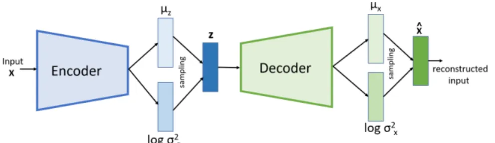
Thevariational autoencoder(VAE) [21] is adeep generative model that aims at uncovering the data generation mechanism in the form of a probability dis- tribution. The VAE is anunsupervised approach that learns a low-dimensional, nonlinear datamanifold from training data without class labels. VAEs achieve this by using two separate but jointly trained neural networks, anencoder and adecoder. The encoder forces the input data through a low-dimensionallatent space that the decoder uses to reconstruct the input.
Given aD-dimensional input x∈RD, the encoder network mapsxinto a latent vector z ∈ Rd (d D). Unlike in a conventional (deterministic) au- toencoder, z is not a single point; instead, the encoder imposes a distribution over the latent variable,qφ(z|x), whereφdenotes all the parameters (network weights) of the encoder. The default choice, also in this work, is a Gaussian qφ(z|x) =N(z|µφ(x),diag
σ2φ(x)
), whereµφ(x) anddiag σ2φ(x)
are de- terministic functions (the encoder network) that return the mean and variance vector (i.e., diagonal covariance matrix) of the latent space given inputx.
The decoder network, in turn, takeszas input and returns a parameterized probability distribution, which is another Gaussian. The decoder distribution is pθ(x|z) =N(x|µθ(z),diag σ2θ(z)
), where µφ(z) anddiag σ2θ(z)
are deter- ministic functions implemented by the decoder network, and where θ denotes the decoder network parameters. Random observations sampled from the de- coder distribution (with fixedz) should then bear resemblance to the inputx.
In the standard VAE, the only sampling that takes place is from the variational posterior distribution of the latent variable. Conceptually, however, it is useful to note that the decoder also produces a distribution of possible outputs, rather a single point estimate, for a given (fixed)z. These outputs will not be exactly the same asxdue to the dimensionality reduction to the lower-dimensionalz- space, but each of the individual elements of thez-space represents some salient, meaningful features necessary for approximatingx.
3.2. VAE training
The VAE is trained by maximizing a regularized log-likelihood function. Let X ={xn}Nn=1 denote the training set, withxn ∈RD. The training loss for the entire training setX,
L(θ,φ) = XN n=1
`n(θ,φ), (1)
decomposes to a sum of data-point specific losses. The loss of thenth training example is a regularized reconstruction loss:
`n(θ,φ) =−Ez∼qφ(z|xn)
h
logpθ(xn|z)i
| {z }
Reconstruction error
+ KL qφ(z|xn)kp(z)
| {z }
Regularizer
, (2)
where E[·] denotes expected value and KL(·k·) is the Kullback-Leibler diver- gence [80] – a measure of difference between two probability distributions. The
reconstruction error term demands for an accurate approximation of xwhile the KL term penalizes the deviation of the encoder distribution from a fixed prior distribution,p(z). Note that the prior, taken to be the standard normal, p(z) =N(z|0,I), is shared across all the training exemplars. It enforces the latent variables z to reside in a compatible feature space across the training exemplars. We use stochastic gradient descent to train all our VAE models.
More training details provided later in4.4.
In practice, to derive a differentiable neural network after samplingz, VAEs are trained with the aid of the so-called reparameterization trick [21]. Thus, samplingzfrom the posterior distribution qφ(z|x) is performed by computing z=µφ(x)+σφ(x)whereis a random vector drawn fromN(z|0,I),µand σare the means and variance of the posterior learned during the VAE training, anddenotes the element-wise product.
3.3. Conditioning VAEs by class label
As said, the VAE is an unsupervised method that learns an encoder-decoder pair, Λ= (θ,φ), without requiring class labels. When used for classification, rather than data reconstruction, we have to condition VAE training with the class label. Here, we use labels yn = 1 (bona fide) and yn = 0 (spoof) to indicate whether or not thenthtraining exemplar represents bona fide speech4. We consider three alternative approaches to condition VAE training, described as follows.
The first,naiveapproach, is to train VAEs similarly as GMMs [68,72,66] — independently of each other, using the respective training setsXbona={xn|yn= 1} and Xspoof ={xn|yn = 0}. VAEs are trained to optimize the loss function described in (2). This yields two VAEs, Λbona and Λspoof. At the test time, the two VAEs are independently scored using (2), and combined by subtracting the spoof score from the bona fide score. The higher the score, the higher the confidence that the test utterance originates from the bonafide class.
Our second approach is to train a singleconditional VAE(C-VAE) [42]
model. In contrast to the naive approach, the C-VAE can learn more complex (e.g., multimodal) distributions by including auxiliary inputs (conditioning vari- ables) to the encoder and/or decoder distributions. In this approach, the label vectorynis used both in training and scoring. Specifically, in our implementa- tion inspired from [81,36], we augmentynto the output of the last convolutional layer in the encoder network and to the input of the decoder network. Section 4.3 describes our encoder and decoder architectures. The training loss (2) is now revised as,
`n(θ,φ) =−Ez∼qφ(z|xn,yn)
h
logpθ(xn|z,yn)i
+ KL qφ(z|xn,yn)kp(z|yn) , (3)
4We use the vector notationynto indicate the correspondingone-hot vector—i.e.,yn= (0,1) to represent bonafide andyn= (1,0) to represent a spoof sample.
(a)Naive VAE. Separate bonafide and spoof VAE models are trained using the respective- class training audio files.
(b) C-VAE. A single VAE model is trained using the entire training examples but with class-label vectors.
(c)AC-VAEextendsC-VAEby augmenting an auxiliary classifier (AC). We include AC in two alternative settings: (i) AC-VAE1: use latent mean vector µz as its input, or (ii) AC-VAE2: at the end of decoder using reconstruction as its input. These are highlighted with dotted lines. At test time we discard the AC.
Figure 2: Different VAE setups studied in this paper.
where, in practice, we relax the class-conditional prior distribution of the latent variable to be independent of the class, i.e. p(z|yn) = p(z) [42]. We perform scoring in the same way as for the previous approach: we pass each test exem- plar x through the C-VAE using genuine and spoof class vectors yn, to give two different scores, which are then differenced as before. Note that yn may include any other available useful metadata besides the binary bonafide/spoof class label. In our experiments on the text-dependent ASVspoof 2017 corpus consisting of 10 fixed passphrases, we will address the use of class labels and phrase identifiers jointly.
Our third approach is to use anauxiliary classifier with a conditional VAE(AC-VAE) to train a discriminative latent space. We userψ(x) to denote the predicted posterior probability of the bonafide class, as given by an auxiliary classifier (AC). And,ψ denotes the parameters of AC. Note that the posterior for the spoof class is 1−rψ(x) as there are two classes. Inspired by [38] and [44], we consider two different AC setups. First, following [38], we use the mean µz as the input to an AC which is a feedforward neural network with a single hidden layer. Second, following [44], we augment a deep-CNN as an AC to the output of the decoder network. Here, we use the CNN architecture from [45].
From hereon, we call these two setups as AC-VAE1and AC-VAE2respectively.
To train the model, we jointly optimise the C-VAE loss (3) and the AC loss. In specific, the loss for thenth training exemplar is
`n(θ,φ,ψ) =α·`n(θ,φ) +β·`n(ψ), (4) where the nonnegative control parametersαandβweigh the relative importance of the regularisation terms during training, set by cross-validation, and where
`n(ψ) denotes the binarycross-entropy loss for the training exemplarxn. It is defined as
`n(ψ) =− yn logrψ(xn) + (1−yn) log(1−rψ(xn))
(5) Note that settingα= 1 andβ= 0 in (4) gives (3) as a special case. At test time we discard the auxiliary classifier and follow the same approach for scoring as in the C-VAE setup discussed earlier. All the three approaches are summarized in Fig. 2.
3.4. Gaussian mixture model (GMM)
Besides VAEs, our experiments include a standard GMM-based approach.
Similar to the VAE, the GMM is also a generative model that includes latent variables. In the case of GMMs, x is a short-term feature vector, and z is a one-hot vector withC components (the number of Gaussians), indicating which Gaussian was ‘responsible’ for generatingx. Letzk= (0,0, . . . ,1,0, . . . ,0)T be a realization of such one-hot vector where thek-th element is 1. The conditional and prior distributions of GMM are:
p(x|z=zk,Λ) =N(x|µk,Σk)
p(z=zk,Λ) =πk, (6)
whereΛ= (µk,Σk, πk)Ck=1denotes the GMM parameters (means, covariances and mixing weights). By marginalizing the latent variable out, the log-likelihood function of a GMM is given by:
logpΛ(x) = logX
z
p(z)p(x|z) = log XC k=1
πkN(x|µk,Σk), (7) used as a score when comparing test featurexagainst the GMM defined byΛ.
At the training stage we train two GMMs (one for bonafide, one for spoof). As maximizing (7) does not have a closed-form solution, GMMs are trained with the expectation-maximization (EM) algorithm [79, 82] that iterates between component assignment (a ‘soft’ version of the true 1-hot latent variablez) and parameter update steps.
3.5. VAEs and GMMs as latent variable models
Given the widespread use of GMMs in voice anti-spoofing studies, it is useful to compare and contrast the two. Both are generative approaches, and com- mon to both is the assumption of the data generation process consisting of two consecutive steps:
1. First, one draws a latent variablezn∼pgt(z) from aprior distribution.
2. Second, given the selected latent variable, one draws the observation from aconditional distribution,xn∼pgt(x|zn),
where the subscript ‘gt’ highlights an assumed underlying ‘true’ data generator whose details are unknown. Both VAEs and GMMs use parametric distribu- tions to approximatepgt(z) andpgt(x|zn). In terms of the ‘z’ variable, the main difference between GMMs and VAEs is that in the former it is discrete (cate- gorical) and in the latter it is continuous. As for the second step, in GMMs, one draws the observation from a multivariate Gaussian distribution corresponding to the selected component. In VAEs, one also samples the reconstructed obser- vation from a Gaussian, but the mean and covariance are not selected from an enumerable set — they are continuous and are predicted by the decoder from a givenz.
Both GMMs and VAEs are trained with the aim of finding model parame- ters that maximize the training data log-likelihood; common to both is that no closed-form solution for the model parameters exists. The way the two mod- els approach the parameter estimation (learning) problem differs substantially, however. As in any maximum likelihood estimation problem, the training ob- servations are assumed to be i.i.d., enabling the log-likelihood function over the whole training dataset to be written as the sum of log-likelihoods over all the training observations. This holds both for VAE and GMM. Let us use the GMM
as an example. For a single observationx, the log-likelihood function is:
logpΛ(x) = logX
z
p(x, z|Λ) =X
z
Q(z)p(x, z|Λ)
Q(z) = log Ez∼Q(z)
"
pΛ(x, z) Q(z)
#
≥Ez∼Q(z)
"
logpΛ(x, z) Q(z)
#
=X
z
Q(z) logpΛ(x, z) Q(z)
(8) where Q(z) is any distribution, and where the inequality in the second line is obtained using Jensen’s inequality [80] (using concavity of logarithm). The resulting last expression, known as the evidence lower bound (ELBO), serves as a lower bound of the log-likelihood which can be maximized more easily.
The well-known EM algorithm [82] is an alternating maximization approach which iterates between updating theQ-distribution and the model parameters Λ (keeping the other one fixed when updating the other one). An important characteristic of the EM algorithm is that, in each iteration, the posterior dis- tributionQ(z) is selected to make the inequality in (8)tight, making the ELBO equal to the log-likelihood. This is done by choosingQ(z) to be the posterior distribution PΛ(z|x) (using the current estimates of model parameters). Im- portantly, this posterior can be computed in closed form. The EM algorithm is guaranteed to converge to a local maximum of the log-likelihood. It should be noted, however, that as the likelihood function contains local maximae [83], global optimality is not guaranteed. The quality of the obtained GMM (in terms of log-likelihood) depends not only on the number of EM iterations, but the initial parameters.
In contrast to GMMs, the posterior distribution of VAEscannotbe evaluated in closed form at any stage (training or scoring). For this reason, it is replaced by an approximate, variational [79] posterior, qφ(z|x), leading to the ELBO training objective of Eq. (2). As the true posterior distribution cannot be evaluated, the EM algorithm cannot be used for VAE training [21]. The ELBO is instead optimized using gradient-based methods. Due to all these differences, it is difficult to compare VAEs and GMMs as models exactly. One of the main benefits of VAEs over GMMs is that they can handle high-dimensional inputs — here, raw spectrograms and CQCC-grams consisting of multiple stacked frames
— allowing the use of less restrictive features.
4. Experimental setup
We describe our experimental setup in this section, including description of the evaluation datasets, features, model architectures and training, and perfor- mance metrics.
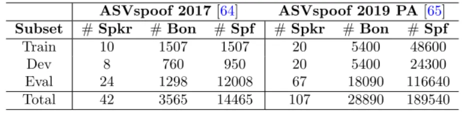
Table 2: Database statistics. Spkr: speaker. Bon: bonafide/genuine, spf: spoof/replay. Each of the three subsets has non-overlapping speakers. The ASVspoof 2017 dataset has male speakers only while the ASVspoof 2019 has both male and female speakers.
ASVspoof 2017[64] ASVspoof 2019 PA[65]
Subset #Spkr #Bon #Spf #Spkr #Bon #Spf
Train 10 1507 1507 20 5400 48600
Dev 8 760 950 20 5400 24300
Eval 24 1298 12008 67 18090 116640
Total 42 3565 14465 107 28890 189540
4.1. Dataset
We use the anti-spoofing dataset that has been released publicly as a result of the automatic speaker verification and spoofing countermeasures5 (ASVspoof) challenge series that started in 2013. We focus on replay attacks that are simple to mount, yet extremely challenging to detect reliably. We use the ASVspoof 2017 (version 2.0) [84] and ASVspoof 2019 PA [65] subconditions as our eval- uation data. Both datasets consist of 16 kHz audio and are complementary to each other. The former consists of real replay recordings obtained by replay- ing part 1 of theRedDots corpus [85] through various devices and environments [86]. The latter dataset consists of controlled,simulated replay attacks, detailed in [87]. Both datasets are split into three subsets: training, development and evaluation with non-overlapping speakers in each subsets. Table2 summarizes the key statistics of both datasets.
4.2. Features and input representation
We consider both CQCC [66] and log-power spectrogram features. We apply a pre-processing step on the raw-audio waveforms to trim silence/noise before and after the utterance in the training, development and test sets, following recommendations in [45] and [76]. Following [84], we extract log energy plus 19- dimensional static coefficients augmented with deltas and double-deltas, yielding 60-dimensional feature vectors. This is followed by cepstral mean and vari- ance normalisation. As for the power spectrogram, we use a 512-pointdiscrete Fourier transform(DFT) with frame size and shift of 32 ms and 10 ms, respec- tively, leading toN feature frames with 257 spectral bins. We use the Librosa6 library to compute spectrograms.
As our VAE models use a fixed input representation, we create a unified feature matrix by truncating or replicating the feature frames. IfN is less than our desired number of feature frames T, we copy the original N frames from the beginning to obtainT frames. Otherwise, if N > T, we retain the first T
5https://www.asvspoof.org/
6https://librosa.github.io/librosa/
frames. The point of truncating (or replicating) frames in the way described above is to ensure meaningful comparison where both models use the same audio frames as their input. This also means that the numbers reported in this paper are not directly7 comparable to those reported in literature; in specific, excluding the trailing audio (mostly silence or nonspeech) after the first 1 second will increase the error rates of our baseline GMM substantially. The issue with the original, ‘low’ error rates relates in part to database design issues, rather than bonafide/spoof discrimination [76,45]. The main motivation to use theT frames at the beginning is to build fixed-length utterance-level countermeasure models, which is a commonly adopted design choice for anti-spoofing systems, e.g. [15,14].
This yields a 100×60-dimensional CQCC representation and a 100×257 power spectrogram representation for every audio file. We use the same number of frames (T = 100) for both the GMM and VAE models. Note that GMMs treat frames as independent observations while VAEs consider the whole matrix as a single high-dimensional data point.
4.3. Model architecture
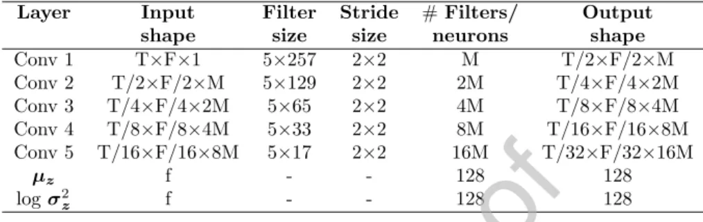
Our baseline GMM consists of 512 mixture components (motivated from [84]) with diagonal covariance matrices. As for the VAE, our encoder and decoder model architecture is adapted from [88]. For a givenT×Dfeature matrix, where T=time frames andD=feature dimension, the encoder predicts the meanµzand the log-variance logσ2z that parameterize the posterior distributionqφ(z|x), by applying a series ofstrided 2D convolutions [89] as detailed in Table3. We use a stride of 2 instead of pooling for downsampling the original input. The decoder network architecture is summarized in Table 4. It takes a 128 dimensional sampledz vector as input and predicts the mean µxand the log-variance log σ2xthat parameterize the distribution through a series oftransposed convolution [89] operations. We use LeakyReLU [90] activations in all layers except the Gaussian mean and log variance layers which use linear activations. We use batch normalisation before applying non-linearity in both encoder and decoder networks.
4.4. Model training and scoring
We train GMMs for 10 EM iterations with random initialisation of param- eters. We train bonafide and spoof GMMs separately to model the respective class distributions as discussed in Section3.4. We train our VAE models (Sub- section3.3) using stochastic gradient descent with Adam optimisation [91], with an initial learning rate of 10−4and 16 samples as the minibatch size. We train them for 300 epochs and stop the training if the validation loss does not improve for 10 epochs. We apply 50% dropout to the inputs of fully connected layers in
7GMMs reported in the literature do not truncate or replicate, and this was done by us for a fair comparison with VAEs.
Table 3: Encoder model architecture. Conv denotes a convolutional operation. T: number of time frames. F: number of feature dimensions. The scalar f is the size of the flattened vector from the last Conv layer output, and represents the number of input units toµz and logσ2z fully connected layers. M=16 for spectrogram inputs and 32 for CQCCs. Conv 5 layer is not applicable for CQCCs.
Layer Input Filter Stride #Filters/ Output
shape size size neurons shape
Conv 1 T×F×1 5×257 2×2 M T/2×F/2×M
Conv 2 T/2×F/2×M 5×129 2×2 2M T/4×F/4×2M
Conv 3 T/4×F/4×2M 5×65 2×2 4M T/8×F/8×4M
Conv 4 T/8×F/8×4M 5×33 2×2 8M T/16×F/16×8M
Conv 5 T/16×F/16×8M 5×17 2×2 16M T/32×F/32×16M
µz f - - 128 128
logσ2z f - - 128 128
our auxiliary classifier. We do not apply dropout in the encoder and decoder network.
4.5. Performance measures
We assess the bonafide-spoof detection performance in terms of the equal error rate (EER) of each countermeasure. EER was the primary evaluation metric of the ASVspoof 2017 challenge, and a secondary metric of the ASVspoof 2019 challenge. EER is the error rate at an operating point where the false acceptance (false alarm) and false rejection (miss) rates are equal. A reference value of 50% indicates the chance level.
In addition to EER, which evaluates countermeasure performance in isola- tion from ASV, we report thetandem detection cost function(t-DCF) [92] which evaluates countermeasure and ASV performance jointly under a Bayesian deci- sion risk approach. We use the same t-DCF cost and prior parameters as used in the ASVspoof2019 evaluation [87], with the x-vector probabilistic linear discrim- inant analysis (PLDA) scores provided by the organizers of the same challenge.
The ASV system is set to its EER operating point while the (normalized) t- DCF is reported by setting the countermeasure to its minimum-cost operating point. We report both metrics using the official scripts released by the organiz- ers. A reference value 1.00 of (normalized) t-DCF indicates an uninformative countermeasure.
4.6. Experiments
We perform several experiments using different VAE setups using CQCCs and log-power spectrogram inputs as described in Subsection3.3. We also train baseline GMMs for comparing VAE performance using the same input CQCC features. While training VAEs with an auxiliary classifier on the µz input, we use 32 neuron units on the FC layer. We do not use the entire training and development audio files for training and model validation on the ASVspoof 2019 dataset, but adopt custom training and development protocols used in
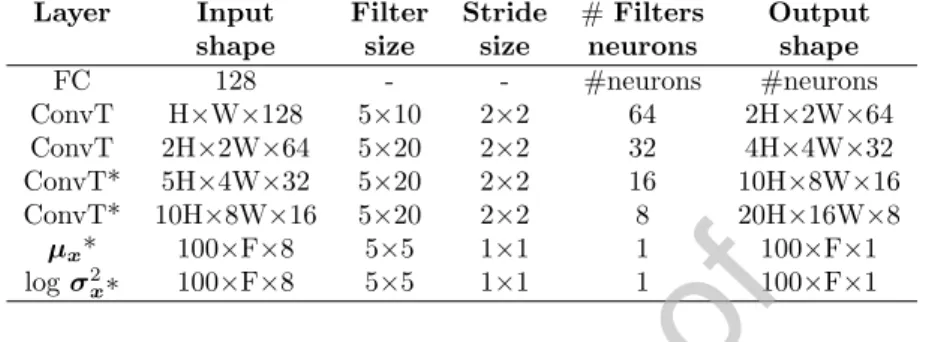
Table 4: Decoder model architecture. ConvT denotes a transposed convolutional operation.
* denotes zero padding operation applied to match the input shape. The Gaussian layersµx
and logσ2x use Conv operation. The initial values of H and W depend on the number of neurons (#neurons) in the FC layer which is 12288 for spectrograms and 2304 for CQCCs.
Layer Input Filter Stride #Filters Output
shape size size neurons shape
FC 128 - - #neurons #neurons
ConvT H×W×128 5×10 2×2 64 2H×2W×64
ConvT 2H×2W×64 5×20 2×2 32 4H×4W×32
ConvT* 5H×4W×32 5×20 2×2 16 10H×8W×16
ConvT* 10H×8W×16 5×20 2×2 8 20H×16W×8
µx* 100×F×8 5×5 1×1 1 100×F×1
logσ2x∗ 100×F×8 5×5 1×1 1 100×F×1
Table 5: EER vs dimension of latent space. Showing the effect of latent dimension on the performance metric for the C-VAE model when trained using CQCCs and spectrograms.
Shown results are on the evaluation set. Shown results are on the ASVspoof 2017 dataset.
Spectrogram CQCC
Latent Dimension EER t-DCF EER t-DCF
8 31.20 0.8642 33.35 0.8584
16 26.88 0.7551 33.74 0.8542 32 36.65 0.9383 30.81 0.7909 64 29.73 0.7650 29.52 0.7325 128 29.43 0.7303 29.27 0.7222 256 29.80 0.7609 28.87 0.6962 512 25.73 0.6662 28.42 0.7033
[76] that showed good generalisation on the ASVspoof 2019 test dataset during the recent ASVspoof 2019 evaluations. Note, however, that all the evaluation portion results are reported on the standard ASVspoof protocols. In the next section we describe our experimental results.
5. Results and discussion
5.1. Impact of latent space dimensionality
We first address the impact of latent space dimensionality on the ASVspoof 2017 corpus. To keep computation time manageable, we focus only on the C-VAE variant. The results, for both CQCC and spectrogram features, are summarized in Table 5. We observe an overall decreasing trend in EER with increased latent space dimensionality, as expected. All the error rates are rel- atively high, which indicates general difficulty of our detection task. In the remainder of this study, we fix the latent space dimensionality tod= 128 as a suitable trade-off in EER and computation.
Table 6: Performance of GMM (baseline) and different VAE models usingCQCCsas input feature. AC-VAE1: augmenting classifier on top of the latent space. AC-VAE2: augmenting classifier at the output of the decoder. Highlighted in bold indicates the best performance among VAE variants.
ASVspoof 2017 ASVspoof 2019 PA
Dev Eval Dev Eval
Model EER t-DCF EER t-DCF EER t-DCF EER t-DCF
GMM 19.07 0.4365 22.6 0.6211 43.77 0.9973 45.48 0.9988
VAE 29.2 0.7532 32.37 0.8079 45.24 0.9855 45.53 0.9978
C-VAE 18.1 0.4635 28.1 0.7020 34.06 0.8129 36.66 0.9104
AC-VAE1 21.8 0.4914 29.3 0.7365 34.73 0.8516 36.42 0.9036
AC-VAE2 17.78 0.4469 29.73 0.7368 34.87 0.8430 36.42 0.8963
5.2. Comparing the performance of different VAE setups with GMM
Our next experiment addresses the relative performance of different VAE variants and their relation to our GMM baseline. As GMMs cannot be used with high-dimensional spectrogram inputs, the results are shown only for the CQCC features. This experiment serves to answer the question on which VAE variants are the most promising, and whether VAEs could be used to replace the standard GMM as a back-end classifier. The results for both the ASVspoof 2017 and 2019 (PA) datasets are summarized in Table6.
Baseline GMM.On the ASVspoof 2017 dataset, the GMM displays EERs of 19.07% and 22.6% on the development and evaluation sets, respectively. Note that our baseline is completely different from the CQCC-GMM results of [84] for two reasons. First, we use a unified time representation of the first 100 frames obtained either by truncating or copying time frames, for reasons explained earlier. Second, we remove the leading and trailing nonspeech/silence from every utterance, to mitigate a dataset-related bias identified in [45]: the goal of our modified setup is to ensure that our models focus on actual factors, rather than database artefacts.
On the ASVspoof 2019 PA dataset, the performance of the GMM base- line8is nearly random as indicated by both metrics. The difficulty of the task and our modified setup to suppress database artifacts both contribute to high error rates. The results are consistent with our earlier findings in [76]. The two separate GMMs may have learnt similar data distributions. Note that the similarly-trained naive VAE displays similar near-random performance.
VAE variants. Let us first focus on the ASVspoof 2017 results. Our first, naive VAE approach falls systematically behind our baseline GMM. Even if
8For sanity check, we trained a GMM without removing silence (and using all frames per utterance) and obtained a performance similar to the official GMM baseline of the ASVspoof 2019 challenge. On the development set, our GMM now shows an EER of 10.06% and t-DCF of 0.1971 which is slightly worse than official baseline (EER = 9.87 and t-DCF =0.1953).
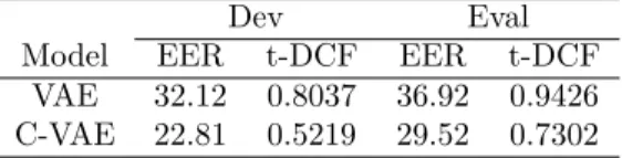
Table 7: Comparing VAE and C-VAE performance on the ASVspoof 2017 dataset using the log power spectrograms as input features.
Dev Eval
Model EER t-DCF EER t-DCF
VAE 32.12 0.8037 36.92 0.9426 C-VAE 22.81 0.5219 29.52 0.7302
both the bonafide and spoof VAE models display decent reconstructions, they lack the ability to retain discriminative information in the latent space when trained in isolation from each other. Further, remembering that VAE training optimizes only a lower bound of the log-likelihood function, it might happen that the detection score formed as a difference of these ‘inexact’ log-likelihoods either under- or overshoots the true log-likelihood ratio — but there is no way of knowing which way it is.
The C-VAE model, however, shows encouraging results compared with all the other VAE variants considered. This suggests that conditioning both the en- coder and decoder with class labels during VAE training is helpful. Supposedly a shared, conditional C-VAE model yields ‘more compatible’ bonafide and spoof scores when we form the detection score. The C-VAE model shows comparable detection performance to the GMM baseline on the development set, though it performs poorly on the evaluation set.
The VAE variants with an auxiliary classifier outperform the naive VAE but are behind C-VAE: both AC-VAE1and AC-VAE2display slightly degraded performance over C-VAE on the evaluation set. While AC-VAE1and AC-VAE2
show comparable performance on the evaluation set, on the development set AC-VAE2 outperforms all other VAE variants in both metrics. This suggests overfitting on the development set: adding an auxiliary classifier increases the model complexity as the number of free parameters to be learned increases substantially. Apart from having to learn optimal model parameters from a small training dataset, another challenge is to find an optimal value for the control parametersαand βin (4).
On the ASVspoof 20199 dataset our C-VAE model now outperforms the naive VAE and the GMM baseline. By conditioning the encoder and decoder networks with class labels, we observe an absolute improvement of about 10%
over the naive VAE on both the development and the evaluation sets. Unlike in the ASVspoof 2017 dataset, the auxiliary classifier VAE now offers some improvement on the evaluation set. This might be due to much larger number of training examples available in the ASVspoof 2019 dataset (54000 utterances)
9We would like to stress that we do not use the original training and development protocols for model training and validation. Instead, we use custom, but publicly released protocols available athttps://github.com/BhusanChettri/ASVspoof2019from our prior work [76] that helped to improve generalisation during the ASVspoof 2019 challenge. However, during test- ing, we report test results on the standard development and evaluation protocols.
in comparison to the ASVspoof 2017 training set (3014 utterances).
It should be further noted that while training models on ASVspoof 2019 dataset, we used the hyper-parameters (learning rate, mini-batch size, con- trol parameters including the network architecture) that were optimised on the ASVspoof 2017 dataset. This was done to study how well the architecture and hyper-parameters generalize from one replay dataset (ASVspoof 2017) to another one (ASVspoof 2019).
The results in Table6with the CQCC features indicate that the C-VAE is the most promising variant for further experiments. While adding the auxiliary classifier improved performance in a few cases, the improvements are modest relative to the added complexity. Therefore, in the remainder of this paper, we focus on the C-VAE unless otherwise stated. Also, we focus testing our ideas on the ASVspoof 2017 replay dataset for computational reasons. Next, to confirm the observed performance improvement of C-VAE over naive VAE, we further train both models using raw log power-spectrogram features. The results in Table7confirm the anticipated result in terms of both metrics.
5.3. Conditioning VAEs beyond class labels
The results so far confirm that the C-VAE outperforms the naive VAE by a wide margin. We now focus on multi-class conditioning using C-VAEs. To this end, our possible conditioning variables could include speaker and sentence identifiers. However, speakers are different across the training and test sets in both ASVspoof 2017 and ASVspoof 2019, preventing the use of speaker condi- tioning. Further, the phrase identities of the ASVspoof 2019 PA dataset are not publicly available. For these reasons we restrict our focus on the 10 common passphrases in the ASVspoof 2017 dataset shared across training, development and evaluation data. The contents of each phrase (S01 through S10) are pro- vided in the caption of Fig. 3. The number of bonafide and spoof utterances for these passphrases in the training and development sets are equally balanced.
We therefore use a 20-dimensional one-hot vector to represent multi-class con- dition. The first 10 labels correspond to bonafide sentences S01 through S10 and the remaining 10 to spoofed utterances. Everything else about training and scoring the C-VAE model remains the same as above, except for the use of the 20-dimensional (rather than 2-dimensional) one-hot vector.
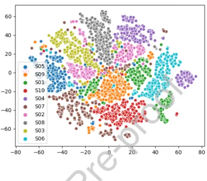
We first visualise how the latent space is distributed across the 10 differ- ent phrases of the ASVspoof 2017 training set. Fig. 3 shows the t-SNE [93]
plots for 10 different utterances in the ASVspoof 2017 dataset. The clear dis- tinction between different phrases suggests that the latent space preserves the structure and identity of different sentences of the dataset. This suggests that choosing the sentence identity for conditioning the VAE might be beneficial to- wards improving performance; such model is expected to learnphrase-specific bonafide-vs-spoof discriminatory cues.
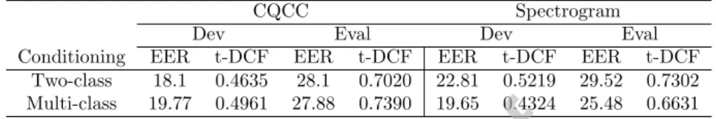
Table 8 summarises the results. The C-VAE trained on spectrogram fea- tures with multi-class conditioning shows a substantial improvement over two- class conditioning. This suggests that the network now benefits exploiting rel- evant information present across different passphrases, which may be difficult
Figure 3: Visualisation of the latent space for 10 different sentences in the ASVspoof 2017 training set by C-VAE with genuine-class conditioning. S01: ‘My voice is my password’. S02:
‘OK Google’. S03: ‘Only lawyers love millionaires’. S04: ‘Artificial intelligence is for real’.
S05: ‘Birthday parties have cupcakes and ice cream’. S06: ‘Actions speak louder than words’.
S07: ‘There is no such thing as a free lunch’. S08: ‘A watched pot never boils’. S09: ‘Jealousy has twenty-twenty vision’. S10: ‘Necessity is the mother of invention’.
from binary class conditioning. For the CQCC features, however, we have the opposite finding: while EER is slightly decreased on the evaluation set with multi-class conditioning, overall it shows degraded performance. One possible interpretation is that CQCCs are a compact feature representation optimized specifically for anti-spoofing. CQCCs may lack phrase-specific information rele- vant for anti-spoofing which is retained by the richer and higher-dimensional raw spectrogram. To sum up, the C-VAE trained on raw spectrograms with multi- class conditioning offers substantial improvement over two-class conditioning in comparison to CQCC input features.
5.4. Qualitative results
A relevant question is whether or not the latent space featuresz have some clear meaning in terms of human or spoofed speech parameters, or any other rel- evant information that helps us derive some understanding about the underlying data. To this end, we analyse the latent space through 2D visualisations using the t-SNE algorithm. We aim to understand how the latent space is distributed
Table 8: Comparing the performance of the C-VAE model trained using two-class and multi- class (10 bonafide and 10 spoof phrases) conditioning. Shown results are on the ASVspoof 2017 v2.0 dataset using CQCC and spectrogram inputs. For two-class conditioning we simply use the class labels yielding 2 dimensional one-hot vector. For multi-class conditioning we use the 10 different passphrases of the ASVspoof 2017 v2.0 dataset. This results in a 20 dimensional one-hot vector (10 for bonafide and 10 for spooof). The results for two-class conditioning (the first row) are included from Table6and7for better readability.
CQCC Spectrogram
Dev Eval Dev Eval
Conditioning EER t-DCF EER t-DCF EER t-DCF EER t-DCF
Two-class 18.1 0.4635 28.1 0.7020 22.81 0.5219 29.52 0.7302
Multi-class 19.77 0.4961 27.88 0.7390 19.65 0.4324 25.48 0.6631
across different speakers and between genders. We do this on the ASVspoof 2019 dataset, as the 2017 dataset only has male speakers. Fig. 4shows t-SNE plots for 5 male and 5 female speakers on the ASVspoof 2019 PA training set chosen randomly.
Subfigures in the first row of Fig.4suggest that the latent space has learned quite well to capture speaker and gender specific information. We further anal- yse bonafide and different attack conditions per gender, taking PA 0082 and PA 0079 — one male and female speaker randomly from the pool of 10 speak- ers we considered. Fig. 4, second row illustrates this. We use letters A-I to indicate bonafide and 9 different attack conditions whose original labels are as follows. A: bonafide, B: ‘BB’, C: ‘BA’, D: ‘CC’, E: ‘AB’, F: ‘AC’, G: ‘AA’, H: ‘CA’, I: ‘CB’, J: ‘BC’. See [65] for details of these labels. From Fig. 4, we observe overlapping attacks within a cluster, and spread of these attacks across different clusters. The bonafide audio examples, denoted by letter A are heavily overlapped by various spoofed examples. This gives an intuition that the latent space is unable to preserve much discriminative information due to the nature of the task, and rather, it might be focusing on generic speech attributes such as acoustic content, speaker speaking style to name a few, to be able to generate a reasonable reconstruction — as depicted in Fig5.
5.5. VAE as a feature extractor
The results shown in Fig. 5 indicate that our VAEs have learnt to recon- struct spectrograms using prominent acoustic cues and, further, the latent codes visualized in Fig. 3indicate strong content dependency. The latent space in a VAE may therefore focus on retaining information such as broad spectral struc- ture and formants that help in increasing the data likelihood leading to good reconstruction. But in spoofing attack detection (especially the case of high- quality replay attacks) we are also interested indetail — the partnot modeled by a VAE. This lead the authors to consider an alternative use case of VAE as afeature extractor.
The idea is illustrated in Fig. 6. We use our pre-trained C-VAE model (with bonafide-class conditioning) to obtain a new feature representation that we dub
Figure 4: t-SNE visualisations of latent space for 5 male and 5 female speaker utterances drawn randomly from the ASVspoof 2019 PA training set. (a)Top left: represents 10 different speaker identities. (b)Top right: male and female clusters (c)Bottom left: distribution of bonafide and attack conditions for a male speaker PA 0082. (d)Bottom right: same as in (c) but for a female speaker PA 0079. A-I indicate bonafide and 9 different attack conditions whose original labels are as follows. A: bonafide, B: ‘BB’, C: ‘BA’, D: ‘CC’, E: ‘AB’, F: ‘AC’, G: ‘AA’, H: ‘CA’, I: ‘CB’, J: ‘BC’. See [65] for details of these labels.
asVAE residual, defined as the absolute difference of the input spectrogram and the reconstructed spectrogram by the C-VAE model. We extract the VAE residual features from all training utterances and train a new classifier back-end (here, a CNN) using these features as input. We adopt the CNN architecture and training from [45]. During testing, we use the CNN output activation (sigmoid activation) as our spoof detection score. Though another recent study also used VAEs for feature extraction [40], our approach is different; the authors of [40] used the latent variable from a pretrained VAE model, while we use the residual of the original and reconstructed inputs.
Table 9 summarizes the results. Numbers in the second row correspond to our proposed approach of using VAE residual features and training a sep- arate classifier. We also include C-VAE results from initial approach (C-VAE as a back-end) from the third row of Table 6for comparison. For contrastive
(a) Audio: D 1000022 with bonafide-class condi- tioning
(b) Audio: D 1000022 with spoof-class condition- ing
(c) Audio: D 1001049 with bonafide-class condi- tioning
(d) Audio: D 1001049 with spoof-class condition- ing
Figure 5: Visualisation of the reconstructed spectrograms by the C-VAE. Shown are the reconstruction of bonafide (D 1000022) and spoof (D 1001049) audio examples using bonafide and spoof class conditioning respectively. The audio examples are taken from the ASVspoof 2017 development set.
Figure 6: VAE as a feature extractor. A pretrained C-VAE model first produces a recon- structed input. The difference of the original and reconstructed input is used as a new feature representation. This feature representation is obtained for the entire dataset and a new clas- sifier (CNN in this case) is trained on the training set features. The development set is used for model validation.
Table 9: C-VAE performance comparison under different settings. Results shown in the first row are taken from Table7second row for comparison — C-VAE trained on spectrograms.
The second row shows results when the same C-VAE model (with bonafide class conditioning) is used as a feature extractor. The third row shows the results when the same CNN classifier is trained on spectrogram input so as to see how it compares with the one trained on VAE residuals. Results shown are on ASVspoof 2017 dataset.
Dev Eval
Features Model EER t-DCF EER t-DCF
Spectrogram C-VAE 22.81 0.5219 29.52 0.7302 VAE residual CNN 13.16 0.3438 17.32 0.4293 Spectrogram CNN 10.82 0.2877 16.03 0.4461
purposes, we train another CNN classifier (using the same architecture) using the original spectrogram directly. Using VAE residuals and training a sepa- rate classifier outperforms the back-end approach on both metrics and on both the development and evaluation sets. The residual approach, however, remains behind the CNN trained directly on the original spectrogram, on the develop- ment set. On the evaluation set, it achieves the lowest t-DCF and displays a comparable EER. The small performance gap (in relative terms) between the development and evaluation sets for the VAE residual approach suggests good generalisation.
Although the proposed VAE residual approach did not outperform the raw- spectrogram CNN, the results obtained are encouraging and show potential for further investigation. In fact, given the similar performance of the original and VAE residual spectrogram features, we interpret the results to mean thatmost of the relevant information for discriminating bonafide and replay utterances (on this data) lies in the residual or ‘noise’ part of the spectrogram. It is noteworthy that heuristic ideas inspired directly by simple visualizations such as Figs. 3 and 5 lead to boosted performance. Finally, recalling our initial motivations, VAE leads to a generative model (unlike CNN) that allows data sampling and obtaining uncertainty of the latent space representation. These favorable properties of VAEs suggest further studies towards more versatile
spoofing countermeasure solutions where the semantics, sanity and stability of the learned feature representation can be easily explored.
6. Conclusions and future work
Inspired by the successful use of GMMs, a classical generative model, as a backend in spoofing detection for ASV, we performed a feasibility study of using an alternative generative model – deep generative VAEs – as a backend classifier. Our first study using two separate VAEs suggests that it is difficult to capture discriminative information when the models are trained using only one-class data. Both the bonafide and spoof VAEs seem to focus on retaining information relevant for data reconstruction while giving less attention on class- discriminative information. As a result, the latent space in both bonafide and spoof VAEs appears to capture common prominent characteristics of bonafide and spoofed speech, making the detection task difficult. Nonetheless, our qual- itative results indicate that both our bonafide and spoof VAEs yield reasonable reconstruction of the input data.
Our second approach of training a single conditional VAE (C-VAE) by con- ditioning the encoder and decoder networks by class-label vectors shows far more encouraging results. The performance of our C-VAE models on both the ASVspoof 2017 and ASVspoof 2019 datasets show remarkable improvement in comparison to the naive VAE approach. Using an auxiliary classifier (AC) did not help much. We did not observe substantial improvement in detection per- formance on the ASVspoof 2017 dataset, though we observed some performance gain on the ASVspoof 2019 dataset, suggesting the importance of training set size for improved generalisation.
Despite different dataset sizes in the ASVspoof 2017 and ASVspoof 2019 datasets, we find that the model hyper-parameters tuned on the ASVspoof 2017 dataset worked quite well when applied on the 2019 dataset, showing con- sistency of our findings with C-VAE models. However, optimisation of network architecture and model hyper-parameters has not been fully explored in the present study, leaving scope for further improvements.
To sum up, based on both the observed detection performance and archi- tecture complexity considerations, from the three VAE back-end variants con- sidered (Fig. 2), the authors recommend potential future work to focus on conditional VAE (C-VAE). In fact, we obtained promising results by further conditioning C-VAE using pass-phrase label. This warrants future studies with other conditioning variables such as speaker identity, gender, channel. Frame- level phone labels obtained through forced alignment procedure might also be interesting with alternative frame-by-frame VAE architectures.
Our primary focus has been to study the feasibility of VAE as a back-end classifier, but we also included a preliminary study on an alternative use case for spectrogram residual feature extraction. The front-end approach demonstrated substantial improvement over the VAE back-end use case, which warrants fur- ther studies. In future work, we also plan to focus on investigating alternative