Inductively coupled resonant sensors can also be used to monitor the properties of materials around the sensor. The author performed the simulations, signal processing and wrote the main parts of the manuscript.
Motivation
The measuring distance of inductive sensors is typically of the same order of magnitude as the dimension of the reader and the sensor coils. The reason for this is that the limitations of the readout electronics during their early development (mid-20thC) made the method cumbersome to use.
Scope
One of the goals of this work is to identify problematic or critical parts of this process and develop technology that will improve the performance of the measurement system in selected applications. On the other hand, the process substances were controlled by sensors whose parameters are changed by the dielectric permittivity of the immediate environment.
Research questions and objectives
Contribution
Organization
Inductively coupled passive resonance sensors
Closely related methods
They suggested that the RFID chips could be used to identify the sensors and to store calibration data. The measurements were therefore in principle similar to the setup used in [26] where an RLC circuit was used to sense the environment.
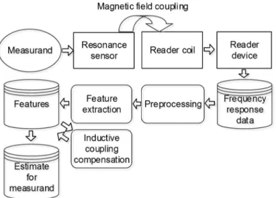
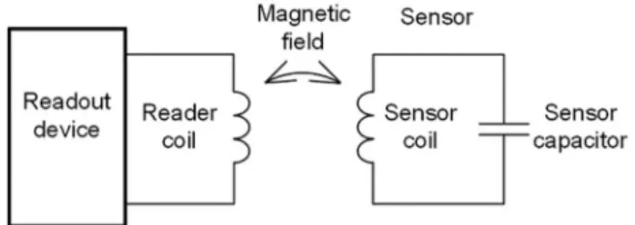
Measurement system
Thus, the impedance of the resonant sensor will have a frequency-dependent effect on the read coil measurement, which means that changes in the measured quantity can be detected by measuring the read coil impedance. The effect of the resonant sensor on the read coil measurement is frequency dependent, so many read devices take measurements at several discrete frequencies.
Resonance sensors
In many applications, the effect of the sensor resistance on the resonant frequency is small and can be ignored. These measurements can be improved by using a moisture sensitive polymer film on top of the sensor [49].
Inductive coupling
Analytical calculations of the mutual inductance for coaxial rectangular spiral coils were presented in [59], and the effects of misalignment were studied in [60]. The effect of the secondary circuit (the resonance sensor) on the primary circuit (the read coil) can be modeled with an equivalent impedance in series with the read coil [27].
Readout devices
The basic concept behind this method is to measure two complex quantities: the current passing through them and the voltage across the unknown component. Subsequently, the voltage across the known impedance can be determined, from which the current supplied to the circuit under test can be calculated. In the network analyzer method, the unknown impedance can be calculated from a reflection coefficient measurement based on measuring incident and reflected signals [64].
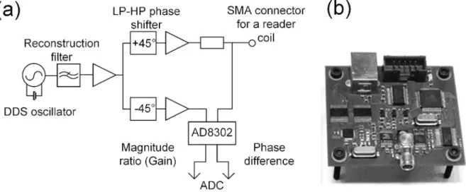
The output signal from the front end is proportional to the real part of the measured impedance. The frequency of the excitation signal is continuously adjusted by the digital signal processing unit.
Signal processing
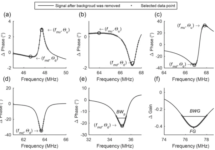
Another frequently used feature is the frequency of the minimum in the impedance phase [28], [32]. These characteristics are believed to have a strong correlation with the resonance frequency of the sensor. The characteristics used to correlate the losses are either the bandwidth of the resonance curve or the Q value [31].
Conversely, the height or magnitude of the resonance curve is correlated with the coupling coefficient. For example, the maximum of the real part of the impedance is eliminated [25].
Inductive coupling compensation methods
The width of the resonance curve can be linked to the losses in the resonant sensor, and especially to the losses in the resistance in the sensor circuit. The information about the height of the resonance curve can be used to compensate for the changes in the resonance frequency estimate. One of the functions used in PCA was the maximum of the real part of the impedance.
The other functions were the frequencies identified from the real and imaginary parts of the impedance. These methods consist of the readout unit, feature extraction methods, and a method to compensate for the effects of changes in the inductive coupling.
Custom-made readout device
However, instead of a real impedance measurement where complex current and voltage are measured, this device simply measures the gain/magnitude ratio and voltage phase shift against a reference channel with an AD8302 detector circuit (Analog Devices) [75]. The device allows fast frequency response measurements that can be used to estimate the resonance frequency of the sensor. This is possible because accurate measurement of the true impedance is not always needed when the measurement is based on the change in the resonance frequency of the sensor.
The software of the device has been designed to allow adjustment and optimization of the frequency parameters. The choice of frequency sweep parameters, such as frequency range and number of data points, is an optimization problem.
Signal processing
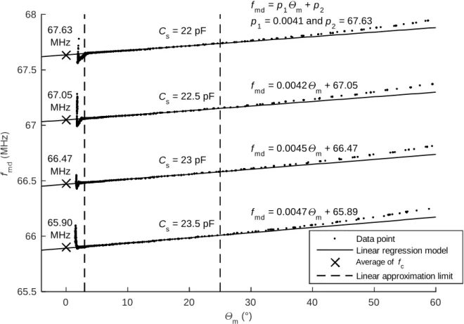
These characteristics can be used as an estimate for the resonance frequency of the sensor. In [P1], the most distinguishable shape in the measured phase data was a peak, so the frequency of the maximum (fmu) of the peak was extracted (Fig. 6a). In that case, the extracted features were the frequency of the minimum (FG) and the width of the dip in the gain curve (BWG).
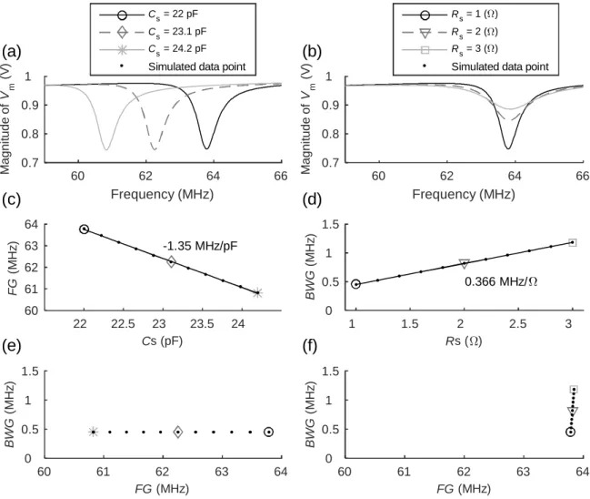
Changes in inductive coupling also affect the relative size of the measured resonance curves (Figures 5a and 5b). Thus, the height of the resonance curve can be used to compensate for possible changes in the inductive coupling.
Discussion on the readout methods
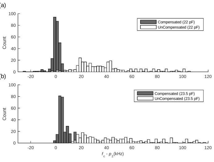
In the second example, the sensor capacitance was 23.5 pF, and the data had 263 valid points. The method apparently reduces the effect of inductive coupling on the extracted resonance frequency estimates. 8b shows a similar histogram for the second case, in which the method still effectively reduces the effect of inductive coupling.
Thus, the compensation causes an error when the resonant frequency of the sensor is shifted far away from the frequency where the tuning process was performed. The compensation method is based on the assumption that the relationship between the height of the resonance curve and the extracted frequency value is linear.
Motivation and goals
Lumped element model
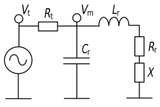
The sensor impedance was modeled with inductance (Ls), capacitance (Cs) and resistance (Rs) using Equation (7). The resistance, (Rt), models the total resistance of the component used to feed current to the reader coil. The parasitic components of the reader coil (Cr and Rr) were added to make the model valid at high frequencies (HF and VHF bands), where most inductively coupled sensors operate.
The parallel capacitances of the reader coils are modeled based on the measurement made with the physical coils. In the tested model, the series configuration of components Rr, Lr and X is in parallel with capacitor Cr.
Simulations
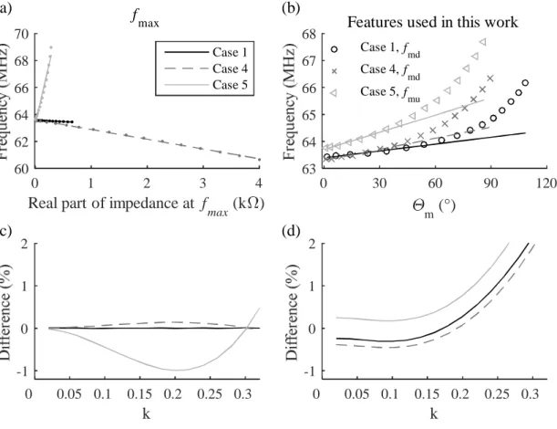
Frequency estimates (fmd, fmu. and fmax) and the corresponding heights of the resonance curves were extracted from the data. In the first configuration, the self-resonance frequency of the reader coil was much higher than the sensor resonance frequency. In the last configuration tested, the self-resonance frequency of the reader coil is lower than the sensor resonance frequency.
The scatter diagram between fmd or fmu and the corresponding Θm. c) The difference between compensated fmax and f0 as a function of the coupling coefficient k. d) The difference between the compensated resonance estimates andf0 as a function of k. The effects of the sensor capacitance and resistance on the resonance curves and the extracted characteristics were studied in a situation where the reader coil configuration (Case 4) approximates the setup used in [P4].
Discussion on the simulations
The changes inCs changed the resonance estimate FG in a fairly linear manner in the tested range (Fig. 12c). The simulated and measured characteristics can be compared when the coupling coefficient in the simulation and the measurement distance in the test situation are changed. In the simulations, the compensation kept the error in the resonance estimate fc low when the inductive coupling was small (Fig. 11d).
The functions FG and BWG are thus good candidates for monitoring the changes in the equivalent capacitance and the equivalent resistance of the sensor in the tested situation. In the compression garment application, the variable capacitors were used to convert the measured pressure to the change in resonant frequency.
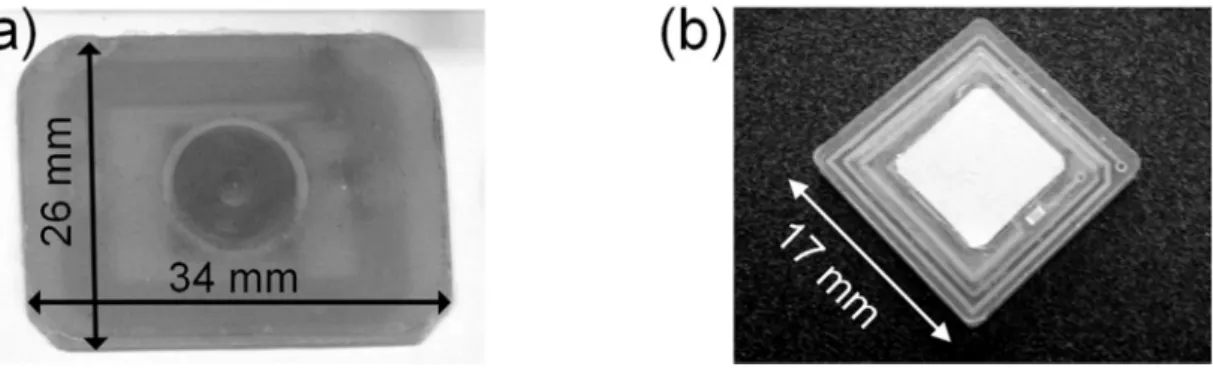
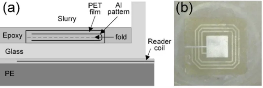
Pressure sensors for compression garments
The pressure generated comes from the elasticity of the garment when it is put on. More examples of pressure responses measured with the second design are given in [91] and [P2]. In this test, the readings of the first prototype were measured as the distance between the read coil and the sensor was changed.
The upper limit of the range is due to the uncertainty in extracting the resonance characteristics from the noise data when the measurement distance is long. Therefore, trade-offs must be made between the measuring distance and the size of the sensor coil.
Monitoring of particle suspensions
The changes of FG were linked to the changes in the real part of the relative dielectric constant of the measured medium. Each added addition of the dispersant decreases the FG and each addition of alumina increases the FG. The data points in the scatter plot illustrate the state of the two monitored manufacturing processes.
The data points illustrate the state of the processes where a portion of either dispersant or alumina was added and mixed into the suspension. The connections between these features and the state of the suspensions in the process need to be further investigated.
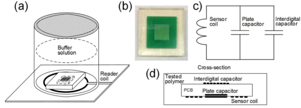
Monitoring of biodegradable polymers in vitro
The results of the reference measurement methods can be found in [P5] and in more detail in [100]. The variation of the estimated frequency of the minimum in the measured fmd phase curve is shown in Fig. The variation in the estimated width of the measured BWp phase curve is illustrated in Fig.
The environment of the encapsulated polymer can be varied and the changes in the characteristics can be continuously monitored online. The measuring distance is largely limited to the dimensions of the coils in the inductive connection. The variations in the inductive coupling can cause significant errors in the resonance frequency estimates.
The compensation method was also applied to one of the readout methods presented in the literature.
![FIGURE 5. a) Resonance curves of a pressure sensor measured using a large reader coil in [P1], b) resonance curves of the pressure sensor tested in [P2], c) resonance curves measured in the polymer degradation measurement, and d) the resonance curves meas](https://thumb-eu.123doks.com/thumbv2/9pdfco/1890462.266628/38.892.118.781.617.964/resonance-pressure-measured-resonance-resonance-degradation-measurement-resonance.webp)