The parameters of the empirical model derived from our theoretical model are estimated with the Smooth Transition Regression (STR) models for the US data. Consequently, changes in the degree of liquidity in the financial markets can be reflected in asset prices if. In the empirical part of the paper, the hypothesis is tested by estimating a smooth transition regression (STR) model with the US data.
A central feature of our approach to modeling the relationship between consumption benefits and liquidity is based on the idea of forming a habit of holding liquid assets. A natural approach to studying habit formation in monetary holdings would be to start with the utility function of form. Furthermore, our hypothesis is that investors' risk aversion depends on the relative proportion of liquid assets in the investor's portfolio, rather than on the absolute level of his cash holdings.
Whether the marginal utility of consumption is a decreasing or increasing function of money balances depends on the value of γ, the measure of relative risk aversion.
DATA
There is also an obvious advantage with our STR specification compared to non-linear models that assume discrete changes between different states, as it allows for a continuum of different levels for the risk aversion among the investors, instead that the value of γ is limited to only two. extreme states. The time series of the logarithmic growth rates of consumption and liquidity are plotted in Figure I.1 in Appendix I. The selection of the transition variables for the estimation of the STR model was limited by some technical difficulties in the estimation procedure.
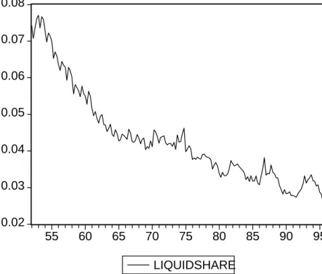
The number of observations of the transition variable in the vicinity of the location parameter (r) was not always large enough to allow the ML procedure to converge to reasonable parameter values. However, it was possible to construct two series to be used as the transition variables. Our first candidate as a transition variable for the STR model was simply the share of the investor's liquid balances from his total portfolio.
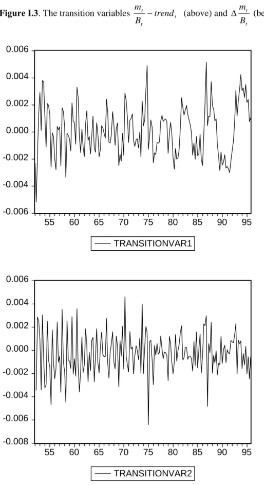
When stationarity was examined using formal unit root tests, the series appeared to be borderline cases between a trend-stationary process and a unit root process around a linear trend. One of the statistical assumptions behind STR models is the stationarity of the transition variable, which suggests removing the deterministic trend from the series of the transition variable before estimation. Consequently, by removing a HP-filtered trend from the weight series of liquid balances of investors' portfolios, we constructed a new series of transition variables: the deviations of the growth rate of liquid balances from their trend.
Our second candidate for the stock return transition variable was the first difference of the share of liquid balances of the total portfolio, i.e. Therefore, we then ask whether consumers have a habit instead of the level of the proportion of liquid assets in their portfolios. Both series, chosen as transition variables, labeled hereafter transition1 and transition2, are plotted in Figure I.3 in Appendix I.
RESULTS
Statistical properties of the model
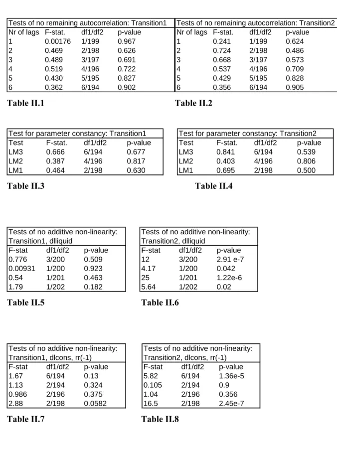
Since the tests clearly suggested residual autocorrelation for both estimated equations, model (6) was respecified by adding a lag of the dependent variable as an additional explanatory variable. As seen in Tables II.1 and II.2 in Appendix II, the null hypothesis of no autocorrelation in the residuals is clearly maintained after lagged stock returns are added to the estimated models. Thus, the stability of the consumption growth rate and liquidity coefficients over time was examined using the test suggested by Teräsvirta (1996) with the null hypothesis of no structural change in the parameter values over the sample period.
The results of the tests are reported in Tables II.3 and II.4 in Appendix II. As can be seen, the null hypotheses of parameter constancy clearly could not be rejected for either of the two specifications of the model, the p-values of the test statistics being equal to or exceeding 0.5 in all slightly different variants of the tests. The null hypothesis of the test is that the linear variables of the estimable model – the growth rate of consumption and the lagged stock return – have no additional non-linear effect on stock return.
The results of tests carried out for several slightly different specifications regarding the nature of the non-linearity are given in Tables II.5 - II.8 in Appendix II. In some cases, the test actually rejects the null hypothesis of no additive nonlinearity, suggesting that linear model variables may also affect stock prices in a nonlinear manner. In principle, the growth rate of consumption could be included in the model in two different ways.
However, the first of the specifications would constrain the non-linear effect of both liquidity and consumption to share the same transition dynamics, including the same transition variable (the share of liquid assets in consumers' total portfolio). However, an attempt to estimate the latter of the two specifications was made by using the growth rate of consumption as a transition variable, following the specification of Kahra and Oikarinen (2003). Overall, although we may leave out some valuable information by limiting the non-linear effect of consumption growth, the main objective of our estimation exercise is still met, as the residuals of the model show no autocorrelation, so the estimated coefficients of the models should still be unbiased .
Estimation results
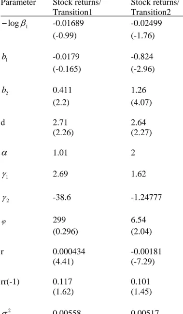
The estimated values of α in the case of the two transition variables considered are 1.01 and 2. The parameter values of most interest to us are the values of γ1 and γ2, the linear and non-linear components of the relative risk aversion measure. Although the sign of γ2 is at least unclear, the large absolute value of the estimate of γ2 implies at least fairly strong nonlinear dynamics of the effect on asset liquidity.
The adjustment dynamics of the transition between regimes was governed by the transition function G( , ; )ϕ r st. The parameters of the function include ϕ, which defines the rate of adjustment, and r which indicates the threshold value for the transition variable. The estimates for the first variables took the values 299 in the case of transition variable 1 and 6.54 in the case of transition variable 2, respectively.
Although the estimates for the threshold values (r) assumed statistically significant values in the case of both transition variables, the estimated size of the estimates was practically zero in both cases. Thus, in the case of the detrended share of liquid assets of the total portfolio of assets as the transition variable, the model implies that the nonlinear portion of γ immediately begins to increase as the share of liquid assets in their portfolios rises above trend. . Similarly, when the change in the rate of liquidity growth was used as the transition variable, the model implies that the faster the share of liquid assets of their.
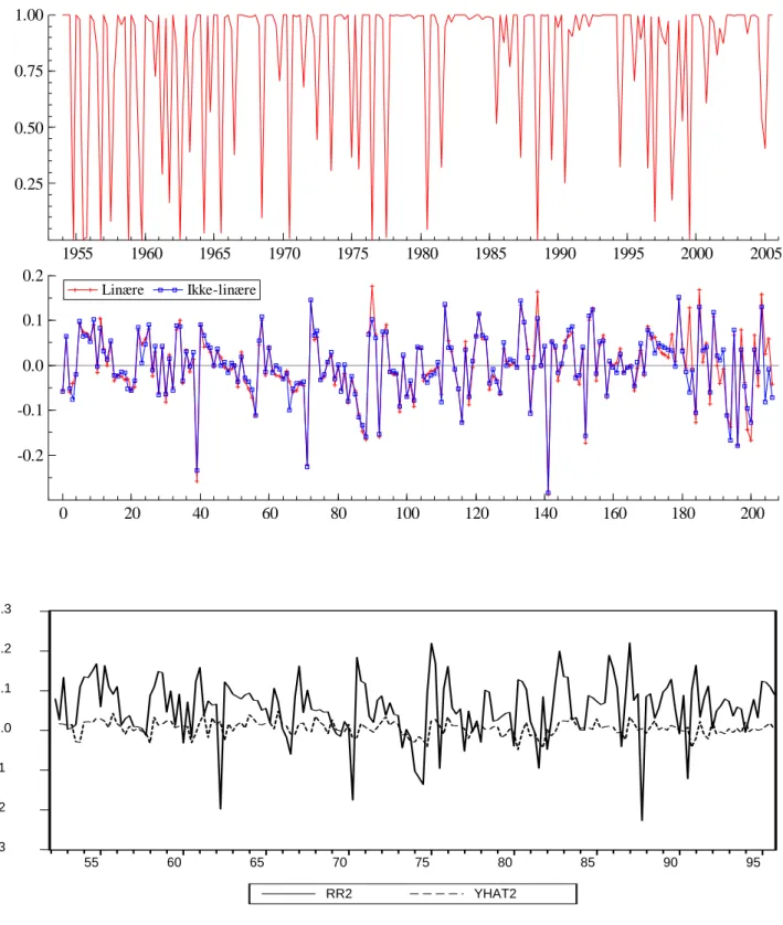
The values for the transition function ( , ; )G ϕ r st are depicted in Figures III.1 and III.2 in Appendix III. Finally, the estimates of the logarithm of the subjective discount factor β obtained from the constant term of the estimated equation deviate statistically from zero in both specifications, obtaining values of 0.01689 and 0.02499. The estimated negative sign of the reduced form coefficient for the money growth rate could be
CONCLUSIONS
The estimated positive sign of the non-linear effect from liquidity to stock returns ( ) seems to contradict this reasoning, since if the explanation holds, then it would be expected that as liquidity in the economy grows, inflationary pressures induced by expanding liquidity in the economy should be stronger, not weaker. An alternative approach to the relationship between money and stock returns has been proposed by Friedman (1970), Nelson (2003) and Congdon (2005), who have argued that consumers or institutional investors may not be willing to increase their holdings in any return assets without a corresponding increase in their holdings of liquid assets. Our estimated positive non-linear impact from liquidity to stock returns after the proportion of liquid balances in the investor's portfolio has exceeded its threshold level can be interpreted as supporting this kind of reasoning.
To discuss these issues, this paper has developed and empirically tested a simple model which predicts a non-linear relationship from the degree of liquidity in the economy to stock returns. The model is based on a version of the consumption-based CAPM, where the consumer's utility function is non-separable in consumption and monetary benefits. The form of the supply function implies that the optimal consumption path partly depends on the consumer's holdings of liquid assets in relation to his constant target for liquidity.
As transitory variables of the STR model, we used two alternative measures of the share of liquid positions in the investor's portfolio. Mainly because of the difficulties in accurately estimating α, the results regarding the parameter we are most interested in, the non-linear component of the risk aversion coefficient, were puzzling in the light of our habit formation hypothesis. On the other hand, the signs of the reduced form model parameter estimates support some previous, albeit tentative, explanations for the observed relationship between liquidity and stock returns: Gallagher and Taylor (2002) and Heimonen (2004) among others. , argued on theoretical and empirical grounds that an increase in liquidity in the economy should decrease rather than increase equity returns.
Determinants of price variability in the stock market American Economic Review, no. Money and Stock Prices: Channels of Influence Journal of Finance, vol. Stochastic consumption, risk aversion and the temporal behavior of asset returns Journal of Political Economy, no. Cash and equity returns in the euro area. No Money, No Inflation - The Role of Money in the Economy Bank of England Quarterly Bulletin, Summer 2002.
Direct Effects of Base Money on Aggregate Demand: Theory and Evidence Journal of Monetary Economics, Vol. The valuation of uncertain income streams and the pricing of options Bell Journal of Economics, no.
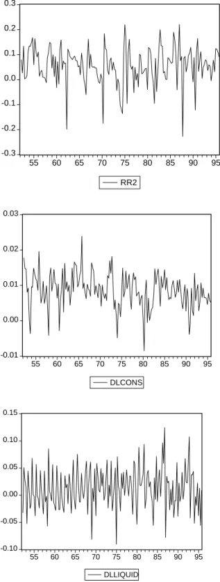
Figure III.1