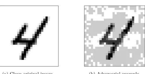
Contradiction attacks on medical imaging data were studied by Finlayson et al. 2021) to identify vulnerabilities in the medical field. Adversarial training and robust upper bounding are compared as strategies for defending against adversarial attacks on three different medical image datasets: a diabetic retinopathy dataset (Kaggle, 2015), a nevus image dataset (ISIC, 2019), and a chest X-ray dataset (Irvin et al., 2019).
Neural Networks
This chapter provides background on adversarial attacks and robust neural network training and discusses related work in this area. There are other versions of stochastic gradient descent, but the method (12) is commonly used to train neural networks.
Adversarial Examples, Attacks and Training
A targeted attack is an attack with a pre-specified desired target, that is, the attacker seeks to obtain a specific output from the model. First order in this context means attacks based on only first-order derivatives, i.e. the gradients of the loss function.
Robustness Certificates and Verification
Katz et al. (2017) extended the standard Simplex method and used a piecewise linear definition of ReLU. Another method by Bertsimas et al. (2021a), Robust Upper Bound (RUB), partitions each layer of a neural network as a sum of convex and concave functions and thus obtains a robust upper bound by further exploiting dual norms.
Adversarial Attacks on Medical Images
The first method, the approximate robust upper bound (aRUB), uses a first-order approximation of the neural network h. Bertsimas et al. (2021b) tested this method along with other boosting methods on a variety of data sets. The same arguments and motivation to prevent financial fraud in the medical field are argued by Ma et al.
A more "realistic" adversarial attack on medical data was investigated by Bortsova et al. 2021), where they used a black-box approach with a surrogate model to construct an attack that was then used on the target model. Bortsova et al.(2021) showed that this kind of attack strategy is successful for medical neural network models, especially if they are pretrained with other publicly available data. Even worse, Hirano et al. 2022) showed that medical deep neural networks are vulnerable to universal adversarial perturbations (UAP).
Then, Section 3.3 presents the modern method proposed by Bertsimas et al. 2021a) is derived and discussed, which provides an approximate upper bound for the saddle problem. Given a classification problem of K different classes with a given data set XN = {xn, yn}Nn=1 N data points and where x∈Rm, m is the number of dimensions and y∈ {1, .., K}, the task of training a robust neural network h is to solve a robust loss problem or a min-max problem with a loss function L and a disturbance δ within Up ={δ :||δ| |p ≤ε}, therefore. Controllability depends on the characteristics of the problem, i.e. the convexity of the objective function and the uncertainty domain.
A Lower Bound
It is clear that the function ϕ(x, z) is continuous but not differentiable with respect to x at the maximum z = 0. The classical Danskin theorem from optimization was loosely used to justify the previous calculations (24) and (25) of the gradient at the maximum, but Danskin (1967) originally formulated a theorem for the minimum and directional derivative that requires the functions to be continuously differentiable, which is not generally true for non-Ural networks. For the context of neural networks, Corollary 1.1 does not always hold, since the ReLU and max-pooling functions are not everywhere continuously differentiable.
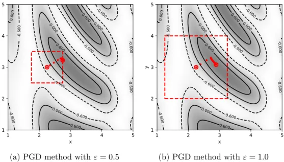
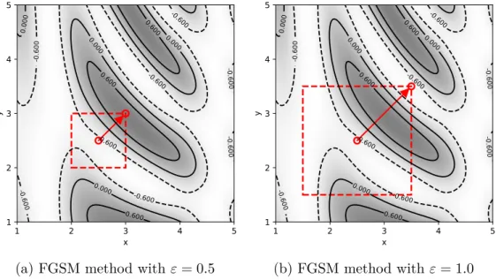
However, as explained by Madry et al. 2018), gradients are local objects and evaluating the gradient at a point that is not continuously differentiable is unlikely during training. Finally, to prove that the gradient descent method moves to the minimum of the loss function for the robust case, the step direction must be decreasing. Basically, the FGSM evaluates the gradient and takes a maximum step until it reaches the boundary of the domain.
Thus, in practice, the lack of differentiability at some points is not a problem when training neural networks. To solve the gradient at a maximum, one must use some method for calculating the maximum, such as FGSM or PGD, which finds feasible and good candidates for the maximizer of the loss function for a given set of weights at that iteration. The computed maximum need not be the true maximizer within the feasible domain.
An Approximate Upper Bound
This linearization of the neural network with respect to the perturbation δ is considered better than linearizing the loss function L, since the loss function is highly nonlinear and neural networks are partially linear close to the original point x. Inserting the linear approximation of the neural networks h into the cross-entropy loss of equation (10) with K yields number of classes. Therefore, the introduction of the concept of the double standard is necessary to solve the maximization problem (52).
The concept of the dual norm is more advanced and more general than presented here with the Euclidean space Rm, but it suffices for the purpose of the derivation to be presented. Finally, the saddle point problem is transformed into an approximate upper bound using a first-order linearization of the neural network and solving the inner maximization via the dual norm. The only difficult task is to estimate the gradient of the neural network with respect to the input.
The details of the models are explained in section 4.3 and the used attacks and their parameters in section 4.4. The first dataset is the diabetic retinopathy dataset (Kaggle, 2015), which is a collection of RGB images of the retina, i.e. the back of the eye. Even after the five classes were grouped into two classes, the data was still unevenly distributed between the two classes and therefore the data was supplemented by rotations and reflections of the images.

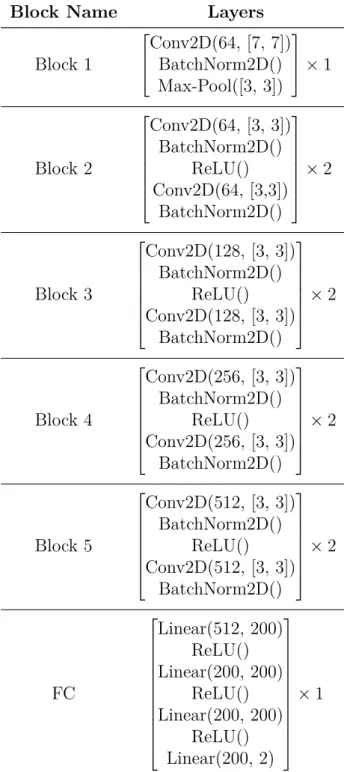
Neural Network
The last fully connected layers are denoted as "Linear()" where the first argument is the input dimension and the second the output dimension. No softmax activation function was used in the last layer since the cross entropy loss or its variant aRUB was used as the loss function. The output dimension of the last layer is two since the neural network is a binary classifier.
Models
Attacks
Hyperparameters and Training
Instead, reasonable parameter values that worked across all models were used for a fair comparison between models. The pretrained weights were obtained directly from PyTorch and they were optimized for the ImageNet dataset. The weights for the last four fully connected layers were initialized with the Xavier initialization method (Glorot and Bengio, 2010), i.e. the weights are uniformly sampled from the interval [−√1m,√1m], where m is the input dimension.
To aid convergence and prevent divergence due to gradient explosion (Goodfellow et al., 2016), gradient clipping was used, where the magnitude of the gradient is bounded by the L2-norm such that ||∇θL(h(x, θ), y)||2 ≤1. aRUB-L1 could not directly converge with the pre-trained ResNet-18 and Xavier weights initialization for perturbation size ε= 0.001. aRUB required initial training of three epochs with one magnitude smaller perturbation size, ie. ε = 0.0001, after which the model could be trained with a desired perturbation size of ε = 0.001 for the remaining seven epochs.
The same types of problems were found with the PGD model for some dataset splits, so the same "hot start" method was performed for both the aRUB models and the FGSM and PGD models.
Implementation
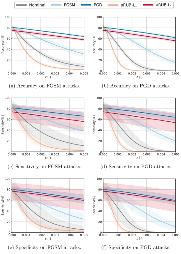
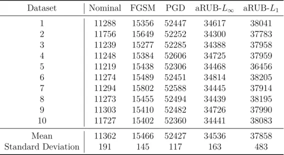
For each data set and each model, 10 different splits were performed on the test and train data sets. Standard metrics of accuracy, sensitivity, and specificity were used to compare the robustness of the models. The training times of the five different models are shown in Table 2 for all 10 partitions of the dataset.
The reason for this is that PGD is an iterative method and requires several steps and computational resources, while aRUB requires only one calculation of the gradient norm of the neural network. The mean performance metrics of accuracy, sensitivity, and specificity are plotted in Figure 8 as a function of perturbation magnitude ε, with the solid line and shaded area representing one standard deviation from the mean, respectively. Performance metrics for FGSM attacks are shown on the left side and PGD attacks on the right side.
For precision, the standard deviation is relatively small, but increases with the size of the perturbation for the aRUB-L1 model to about 10%. For specificity, the standard deviation is greater than for sensitivity and precision for the aRUB-L1 model, indicating that there is a difference between the different performance data partitions. The solid line corresponds to the mean of 10 data bins and the shaded area corresponds to one standard deviation of the mean.
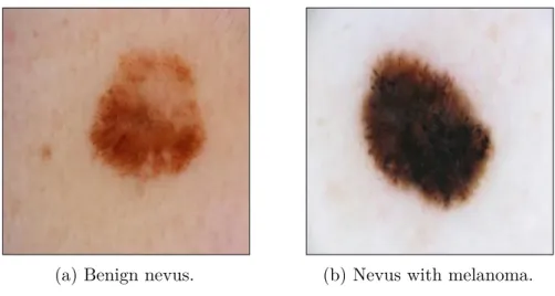
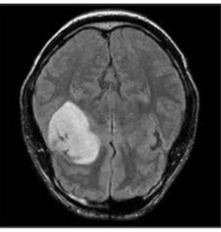
Nevus Dataset
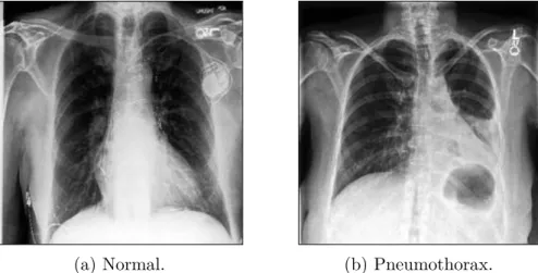
Chest X-ray Dataset
Discussion
The most likely explanation for this is that since the attack uncertainty set was U∞, the appropriate double rate in the aRUB formulation is then the L1 rate, not the L∞ rate. Regularizers are commonly used in training neural networks to avoid overfitting, and here the model probably benefits from a larger value of the norm (regulator) for adversarial attacks. Another interesting observation is that the addition of data does not appear to have affected the robustness of the models.
The results showed good robust performance for both the PGD and the aRUB-L1 model, with a slightly better performance of PGD. The weights of the last fully connected layers were trained together with the parameters of the convolution layer, which differs from the model distillation training proposed by Papernot et al.(2016a). However, with the right model distillation framework, this idea of robusting the last fully connected layers with the exact robust upper bound can be part of further future development and further development of the robust optimization approach.
Another possible future research idea of the robust optimization approach could be to implement the aRUB on different loss functions. The basic idea of the aRUB was to linearize the neural network h instead of the loss function L with respect to the disturbance δ. The training metrics monitored during the training of the neural network are the loss and accuracy evaluated for the training and test set, respectively.
The colored thinner lines correspond to one of the 10 sets used and the thicker black line corresponds to the average of the training data. The colored thinner lines correspond to one of the 10 sets used and the thicker black line corresponds to the average of the training data.