1 The total variation

These lecture notes were prepared for the summer school on sparsity, hosted in Linz, Austria, by Massimo Fornasier and Ronny Romlau, during the week of August. They include work done in collaboration with Vicent Caselles and Matteo Novaga (for the first theoretical parts), and with Thomas Pock and Daniel Cremers, for the algorithmic parts.

Why is the total variation useful for images?

The Bayesian approach to image reconstruction

Everyone is, of course, thanked very much for the work we have done together so far – and for the work that still needs to be done. It represents the idea we have of perfect data (in other words, the model for the data).

Variational models in the continuous setting

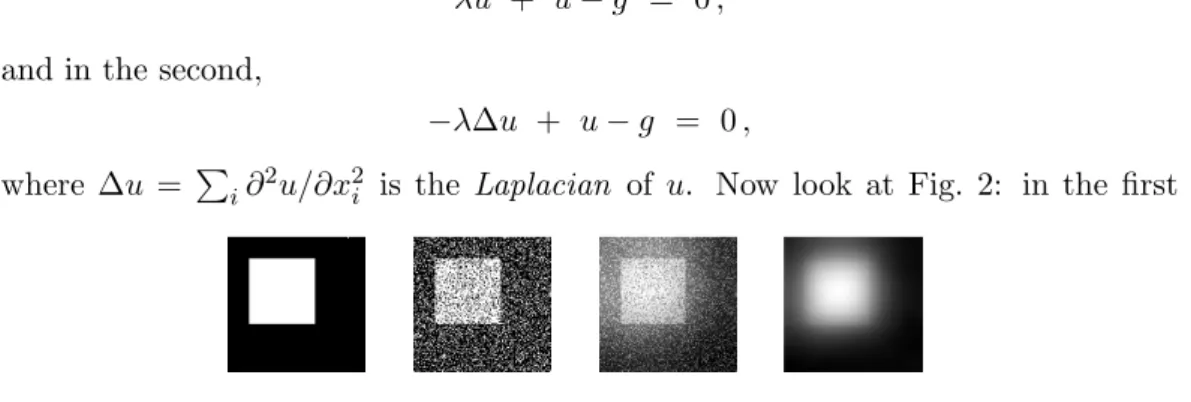
The advantage of these choices is that the corresponding problem to solve is linear, in fact the Euler-Lagrange equation is for the minimization problem in the first case. This is the famous "Mumford-Shah" function, the study of which has generated a lot of interesting mathematical tools and problems in the last 20 years, see esp.

A convex, yet edge-preserving approach

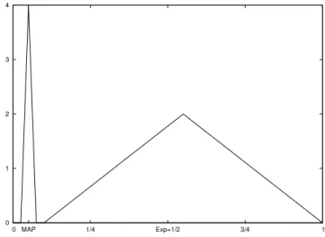
This tells us that a minimizer, if it exists, must be ≤1 a.e. 1 here is the maximum value of g). In particular, in the last case λ≥1/2, we deduce that the only possible minimizer is the function u(t)≡1/2.

Some theoretical facts: definitions, properties

• Definition
• An equivalent definition (*)
• Main properties of the total variation
• Functions with bounded variation

It turns out that this definition is consistent with the more classical definition of total variation, which we will present below, in Definition 1.1 (see inequality (2) and Them. 1). When Ω6=RN, this theorem is shown by a subtle version of the classical proof of the Meyers-Serrin theorem [53], see for example [40] or [7, Thm.

The perimeter. Sets with finite perimeter

Definition, and an inequality

The reduced boundary, and a generalization of Green’s formula 19

The quantity ∂∗E is called the “reduced” limit of E (the “true” definition of the reduced limit is a bit more precise and the exact quantity a bit smaller than ours, but still (10) is true with our definition, see [ 7 , ch. 3]). One shows that this "reduced limit" is always, as in this simple example, a rectifiable set, that is, a set that can be almost completely covered by a countable union of C1hypersurfaces, up to a set of HausdorffHN−1 measure zero: there exist (Γi)i≥1, hypersurfaces with regularityC1 such that.

The co-area formula

The derivative of a BV function (*)

One can show that U is a correctable set (see Section 1.3, Eq. 12)), in fact, it is a countable union of correctable sets since it can always be written. On the other hand, it is continuous as a uniform limit of continuous functions, so Du has no jump parts.

The Rudin-Osher-Fatemi problem

• The Euler-Lagrange equation
• The problem solved by the level sets
• A few explicit solutions
• The discontinuity set
• Regularity

Now let's show that, as in the previous section, the level sets Es = {u > s} solve a given variational problem (of the form (16), but with g(x) replaced by an s-dependent function) . For X a Hilbert space, the subgradient of a convex function F : X →(−∞,+∞] is the operator ∂F that maps x∈X to the (possibly empty set). Ωz ∇u dx for all smooth u with compact support; ii.) the above also applies to u∈H1(Ω) (not compactly supported), in other words z·νΩ = 0 on∂Ω in the weak sense. In all cases we see that z must be orthogonal to the level sets ofu (of|z| ≤1 and z·Du=|Du|), so that −divzi is still the curvature of the level sets.

Now we show that the jump group of uλ is always contained in the jump group of g. The same idea, based on the control over curvature of level sets provided by (ROFs), gives further continuity results for solutions of (ROFs).

Basic convex analysis - Duality

Convex functions - Legendre-Fenchel conjugate

It is essential here that F, G are convex, since we will focus on convex optimization techniques, which can produce quite efficient algorithms for problems of the form (39), providing F and Ghave a simple structure. It is well known and easy to show that if F is twice differentiable at every x∈X, then it is convex if and only if D2F(x)≥0 at every x∈X, in the sense that for every x, y,P . IfF is of class C1, one has that F is convex if and only if. Therefore, we have F ∈ Γ0 if and only if epiF is closed, convex, nonempty, and different from X×R. Another standard fact is that in finite dimension, every convex F is locally Lipschitz in the interior of its domain.

It is also appropriate if F is convex and proper, as we will see shortly: therefore it maps Γ0 into itself (and in fact, onto).

Subgradient

Monotonicity The subgradient of a convex function F is an example of a "monotonic" operator (in Minty's sense): evident from the definition we have for each x, y and any p∈∂F(x),q ∈∂ F(y),. This is an essential property, since many algorithms were designed (mostly in the 1970s) to find the zeros of monotone operators and their many variants.

The dual of (ROF )

We conclude this section by introducing more generally the "proximal" operator associated with a function F ∈Γ0.

Gradient descent

Splitting, and Projected gradient descent

This is an example of "splitting" (first introduced by Douglas and Rachford, see for example [48] for a general form): one successively solves one step of the gradient descent of F (in an explicit way ), and one step of the gradient descent of G (in an implicit way), to obtain a "full" gradient descent of F+G. In caseGis, as here, a characteristic function and (I+h∂G)−1is a projection), then this reduces to a "projected gradient algorithm": one does one explicit step of descent in F, and reprojects then the point on our constraint. Again, this algorithm is quite slow, but it is interesting to understand the intuitive idea behind it.

Now, suppose x = xn and we replace the minimization of F, at step n, by the minimization of QL(y, xn) w.r.y. This is one way to interpret that algorithm, and it provides a natural way to extend it to F+G minimization: indeed, we can now let .

Improvements: optimal first-order methods

Augmented Lagrangian approaches

Primal-dual approaches

The scheme, as it is, is proposed in a paper by Zhu and Chan [73], with an interesting (and very efficient) speedup obtained by changing the time steps, but unfortunately no proof of convergence exists not. We recently provided in [63] the following variant, inspired by a paper by L. Note that the algorithm can also be written with a variable ¯yin instead of ¯x, and recursively first inx, then iny.). It is a slight variant of "extragradient" algorithms (first proposed by G. Korpelevich [44]) and known to converge.

This algorithm has recently been presented as a special case of a more general algorithm in [33], and a proof of convergence is also given there. In fact, we can show convergence of the iterates to a solution in finite dimension, while in the general case we mimic the proof of [57], where A.

Graph-cut techniques

However, we will see in the next section 3.7 that the convergence can apparently be improved by changing the time steps and relaxation parameters, as suggested in [73], although we do not have a clear explanation for this (and it is possible that this speedup is problem dependent is, contrary to the result of Theorem 12). It is easy to check that this approximation is useful for many variants of (38) or similar discretizations of (16). We will not describe this approach in these notes, and refer to [23], and the references therein, for details.

Comparisons of the numerical algorithms

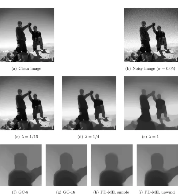
Finally, we note that since graph cut algorithms compute the exact solution with respect to a discretized (8 Bit) solution space, their results are not directly comparable to those of the continuous optimization algorithms. The first row shows the clean and noisy input images and the second row shows results for different values ​​of the regularization parameterλ. For a 16-connected graph, the results are very close to those of the continuous algorithms.

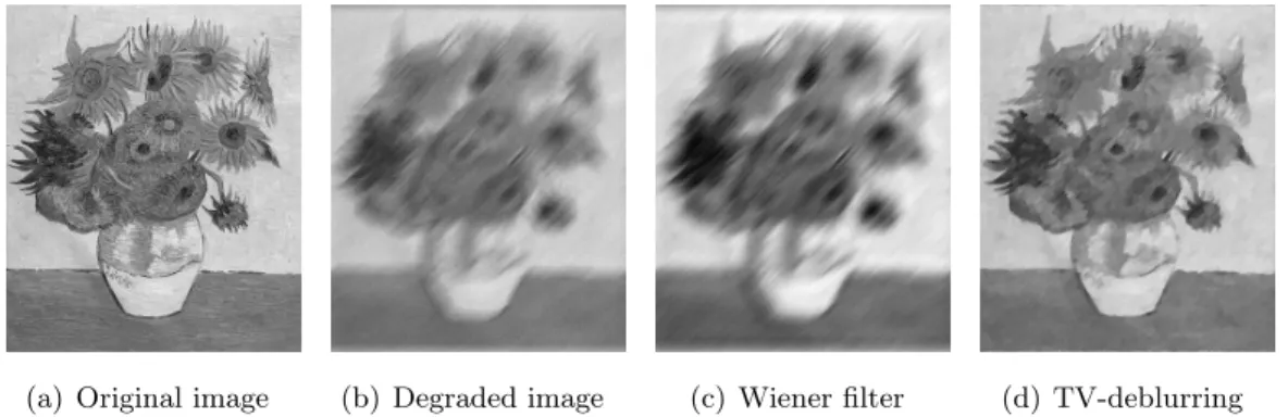
Initially, one can observe that for larger values ​​of λ the problem becomes more difficult for all algorithms. The standard (ROF) model can easily be extended for image blurring and digital zoom. 60) where Ω⊂R2 is the domain of the image and A is a linear operator.

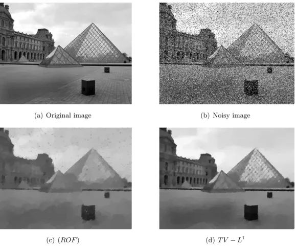
Total variation with L 1 data fidelity term

An elaborate Lagrangian method has recently been proposed to calculate the exact minimization of the TV −L1 model [32]. To apply the proposed modified extragradient method to solve the TV−L1 model, we rewrite it in terms of a saddle point problem (55). On the other hand, the TV −L1 model does not give too much weight to the outliers and thus leads to much better results.

Variational models with possibly nonconvex data terms

Convex representation

Let's start by considering the subgraph of the function u(x), which is the set of all points that lie below the function value u(x). In the following it will appear that by choosing an appropriate vector fieldφ, F(u) can be expressed as the maximum flux of φthrough Γu. Remarkably, this works for functions f(x, u(x),∇u(x)) with a fairly arbitrary behavior in u(x) (albeit continuous, in that variable).

Using (68) and the definition of the indoor unit normal (67), the flux can be rewritten as. 4And in fact it is not entirely surprising if you first think of the case N=0.

Convex relaxation

Numerical resolution

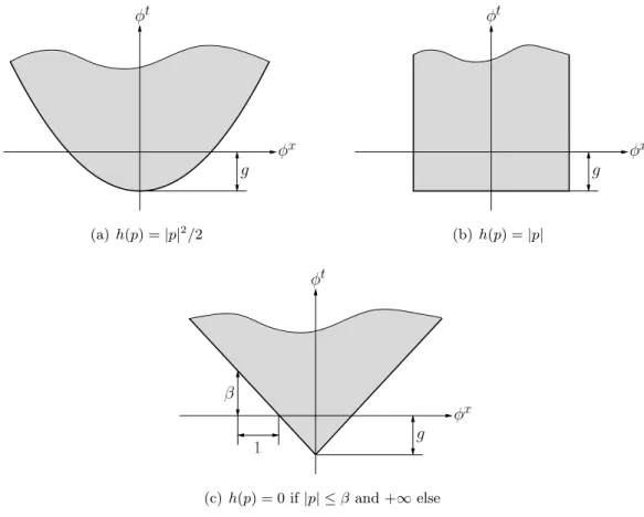
Then, after computing the solution of (83), the projection solution is given by. a) Left input image (b) Right input image (c) “True” disparity. Lipschitz Constraint An advantage of this approach is that a Lipschitz constraint is quite easy to implement. Then, the convex conjugate of simpleh∗(q) =L|q|, and we only need to know how to project q0 onto the convex cone {qt ≥L|qx|}, see Fig.

Example Figure 14 shows three examples of stereo reconstruction using the three different regularizers described above. As expected, the Lipschitz constraint limits the slope of the solution, while the quadratic constraint also smooths.

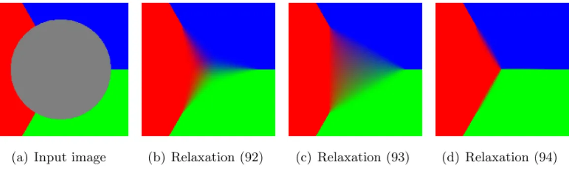
The minimal partition problem

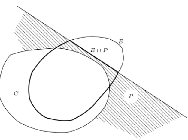
This construct is related to the theory of “paired calibration”, introduced in the 1990s by Lawlor-Morgan and Brakke [ 46 , 18 ]. This is done by alternative projections, following Dykstra's algorithm for projection onto the intersection of convex sets [17]. The next figure 16 shows an example of a minimization of (91) carried out according to this method. The numerical calculations have been performed on a GPU.).

Development of characteristic functions of convex sets in the plane with minimizing total variational flow. On the Douglas-Rachford splitting method and the proximal point algorithm for maximal monotone operators.