HAL Id: hal-03284753
https://hal.inria.fr/hal-03284753
Submitted on 12 Jul 2021
HAL
is a multi-disciplinary open access archive for the deposit and dissemination of sci- entific research documents, whether they are pub- lished or not. The documents may come from teaching and research institutions in France or abroad, or from public or private research centers.
L’archive ouverte pluridisciplinaire
HAL, estdestinée au dépôt et à la diffusion de documents scientifiques de niveau recherche, publiés ou non, émanant des établissements d’enseignement et de recherche français ou étrangers, des laboratoires publics ou privés.
Matthieu Gschwend
To cite this version:
Matthieu Gschwend. A 3D vertex centered CENO scheme for advection. [Research Report] RR-9415,
Inria Sophia Antipolis - Méditerranée. 2021, pp.37. �hal-03284753�
ISSN0249-6399ISRNINRIA/RR--9415--FR+ENG
RESEARCH REPORT N° 9415
2021
Project-Team Ecuador
centré sommet pour l’advection
Matthieu Gschwend
RESEARCH CENTRE
SOPHIA ANTIPOLIS – MÉDITERRANÉE 2004 route des Lucioles - BP 93 06902 Sophia Antipolis Cedex
Matthieu Gschwend
∗Équipe-Projet Ecuador
Rapport de recherche n° 9415 — 2021 — 37 pages
Résumé : Nous présentons un schéma volumes-finis avec une reconstruction quadratique de la solution pour une équation de type hyperbolique 3D sur des maillages non-structurés formés de tétraèdres. Ce schéma est une adaptation au contexte centré-sommet du schéma CENO. Ce travail a été financé par l’Agence Nationale de la Recherche dans le cadre du projet NORMA, contrat ANR-19-CE40-0020-01.
Mots-clés : Volumes finis, Ordre élevé
∗Université Côte d’Azur,INRIA-Ecuador,B.P.93,06902 Sophia-Antipolis, FRANCE,matthieu.gschwend@inria.fr
a 3D hyperbolic equation on structured unstructured meshes formed of tetrahedra. This scheme is an adaptation of the CENO scheme to the vertex-centered context.This work was supported by the ANR project NORMA under grant ANR-19-CE40-0020-01.
Key-words: Finite Volume, higher order
Table des matières
1 Introduction 4
2 Basic scheme 4
2.1 Continuous advection model . . . 4
2.2 k-exact finite volume . . . 5
3 Two-step reconstruction 6 4 Defining the reconstruction molecule 7 4.1 Algorithmics . . . 7
4.2 Examples . . . 10
5 Polynomial reconstruction 10 5.1 Quadratic polynomial reconstruction . . . 10
5.2 Cubic polynomial reconstruction . . . 13
5.2.1 General case . . . 13
5.2.2 Partition case . . . 21
6 Flux evaluation 22 6.1 Flux evaluation for third-order accuracy . . . 22
6.2 Flux evaluation for fourth-order accuracy . . . 23
7 Time advancing 25 7.1 Explicit time advancing . . . 25
7.2 Implicit time advancing . . . 25
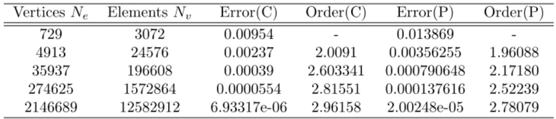
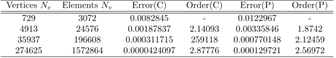
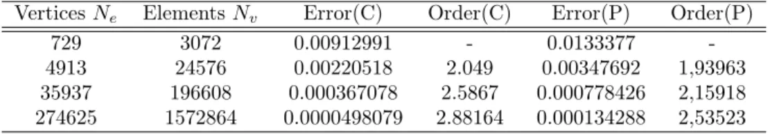
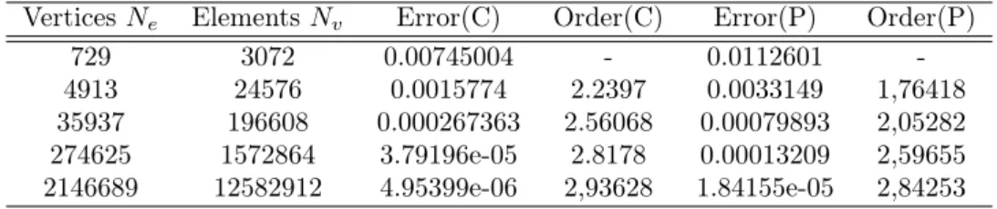
8 Numerical validation of an advection kernel 25 8.1 Third-order validations . . . 25
8.2 Fourth-order validation . . . 28
8.3 Computational cost for the third-order version . . . 28
8.3.1 With centered molecules . . . 28
8.3.2 With partition . . . 29
9 Numerical validation in a CFD code 29 9.1 SOD tube test case . . . 29
9.2 Half cylinder flow . . . 32
9.2.1 Mach number analysis . . . 32
9.2.2 Pressure analysis . . . 34
9.2.3 Entropy analysis . . . 35
9.3 Cylinder flow CPU analysis . . . 36
10 Concluding remarks 36
11 Acknowledgements 36
RR n° 9415
1 Introduction
We are interested in the derivation of dissipative higher-order methods for CFD. By dissipative, we mean that we shall address advective models for which the option of no numerical dissipation can cause an important lack of robustness. Due to this, most CFD, particularly compressible CFD, approximations will involve dissipation devices, mainly based on the introduction of Riemann solvers as initiated by Godunov.
Most high-order approximation schemes like Discontinous Galerkin [4, 7, 8, 15], ENO [3, 9, 11, 13] or distributive schemes [2] use kth-order interpolation or reconstruction and are k- exact. Interpolation and reconstruction are two approximation mappings, the errors of which need to be analysed. Most analyses are inspired by the Bramble-Hilbert principle, saying that an approximation which is exact forkth-order polynomial is a(k+1)th-order accurate approximation.
Demonstrations can be found in the fundamental paper [6]. Later, when considering reconstruction- based schemes, see [10], the authors refered to the Taylor series. A re-visitation in [1] establishes the link with [6].
The goal of the presented research is to study a 3D version of a third-order accurate and a fourth-order accurate Central Essentially Non-Oscillatory central (CENO) approximation, based on a quadratic polynomial reconstruction (then CENO2). These scheme are inspired by the CENO proposition of Groth and coworkers, see [12]. We prealably transpose them to a vertex formulation, as in [5]. The extension to 3D is described of an advection model. In order to save CPU, we examine a new reconstruction molecule for this scheme.
The efficiency of a high order scheme does not depend solely of its order of convergence. In the case of finite-volume based approximations, we have to evaluate for a given mesh the number of degrees of freedom, the reconstruction/interpolation effort, and the number of finite volume fluxes to be evaluated. By comparison with second-order schemes, e.g. MUSCL, vertex CENO needs reconstructions, and, of most cost, high-order integrated fluxes at finite volume interfaces.
By comparison with a discontinuous Galerkin of degree three (for fourth order), an DG3 element contains 20 d.o.f. and need four high-order integrated fluxes. The DG3 element can be split in 27 DG1 orP1elements. Counting 6 elements for a vertex, this shows that a vertex CENO of degree 3 will have 27/6=4.44 d.o.f. on the same DG3 mesh, but with 14*27/6=62 fluxes to evaluate. We shall see that this last figure is still increased due to the special geometry of vertex interfaces.
Then it appears that the Achille neel of vertex CENO is the computational cost of the fluxes. The smaller number of d.o.f. can be advantageous in case of implicit time advancing. The treatment of discontinuity can also be easier that for DG. And for the user, a given mesh ofnvertices will not lead to much more thannd.o.f.
We start this report with a presentation of the basic scheme, a discussion of reconstruction molecules, of quadratic and cubic polynomial reconstruction, of fluc evaluation, of time advancing, and the report is completed with a few numerical experiments.
2 Basic scheme
2.1 Continuous advection model
We consider the following advection model :
∂u
∂t(x, y, z, t) +∇ ·f(u(x, y, z, t)) = 0 (1)
where initial and boundary conditions are : u(x, y, z,0) =u0(x, y, z)
u(x, y, z, t) = Φ(x, y, z, t) for(x, y, z)∈∂Ω (2) where (x, y, z) ∈ Ω with Ω an open subset of R3. For t ≥ 0, u : Ω×R∗+ −→ R. The flux f(u(x, t)) = (f1(u(x, t)), f2(u(x, t)), f3(u(x, t)))t withfi∈C1(R,R).
In this report, we restrict toconstant-velocity advection:
f(u(x, t))) = (V1(u(x, t)), V2(u(x, t), V3(u(x, t)))t with(V1, V2, V3)∈R3. (3) The velocity V = (V1, V2, V3)t being given. Then the boundary conditions for well-posedness are :
u(x, y, z, t) = Φ(x, y, z, t) forV·n<0∈∂Ω (4) oùnest la normale extérieure locale de la celluleCi.
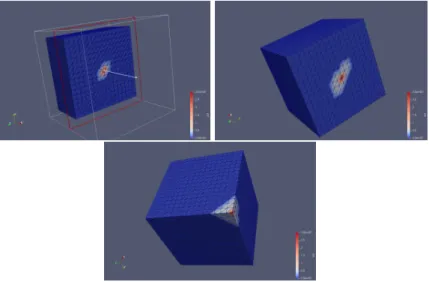
The computational domain Ω is partitioned in dual vertex-centered finite-volume cells Ci
around vertices i, limites by triangular facets IgG, connecting mid-edge, centroid of face and centroid of tetrahedra, Figure 1. As a result, the cell is made of a certain number of minitets
Figure1 – Dual cells from tetrahedras. Left, view of the boundary of cellCi(i: highest vertex in the figure) with a tetrahedronijkl. The cellCiaround vertexiis made of all subtetrahedrasigGIwhereI is the middle of a neiboring edge,gthe centroid of a tetrahedron faceijk containingiI,Gthe centroid of a tetrahedron containing the same faceijk. Right, intersection of the boundaries of celliand cellj, on the facet of which is integrated the flux between celliand cellj.
included in the neigboring tetrahedras, each tetrahedron of the mesh being split into24of these minitets. For the finite volume formulation, we integrate the above equation 1 on cell Ci and apply the Green formula :
d dt
Z
Ci
u(x, y, z, t)dxdt+ Z
∂Ci
f(u(x, y, z, t))·nds= 0 which becomes :
d dt
Z
Ci
u(x, y, z, t)dxdt+ X
k∈V(i)
Z
∂Ci∩∂Ck
f(u(x, y, z, t))·nds= 0. (5) whereV(i)is the set of vertices j directly neighboringi,i.e.sharing an edge ij.
2.2 k-exact finite volume
The fielducan be projected in a spatially-discrete fieldu¯= (u1, .., uncell)defined by :
¯ ui=
Z
Ci
udΩ.
Let Pj(¯v) a set of polynomials defined on Ω, with index j possibly identical to i. A central assumption is thek-exact reconstruction assumption:
For any polynomial v of degree k, Pj reconstructs exactly v. (6)
RR n° 9415
We havePj(¯u) =ufor anyj. Due to the k-exactness of the reconstruction we have : Z T
0
Z
Ci
∂Pj(¯u)
∂t dΩdt+ Z T
0
Z
∂Ci
f(Pj(¯u))·ndσdt= 0. (7) In order to build a spatially discrete problem with a spatially discrete unknown, we introduce a vectorvi(t)such that :
¯ vi(0) =
Z
Ci
u(x,0)dΩ ∀i. (8)
Vectorvi(t)is the semi-discrete solution of thek-exact reconstruction finite volume : Find vi(t)such that (8) holds together with :
RT 0
R
Ci
∂Pi(¯v)
∂t dΩdt+RT 0
R
∂Cif(Pi(¯v))·ndσdt= 0.
If we add the followingconservation assumptionconcerning the reconstructionP : Z
Ci
Pi(¯v)dΩ =meas(Ci)¯vi (9) We get a finite-volume formulation :
Find vi(t)such that (8) holds together with : RT
0
R
Ci
∂v¯i
∂tdΩdt+RT 0
R
∂Cif(Pi(¯v))·ndσdt= 0.
(10)
This finite volume spatial discretization isk-exact, that is satisfies :
If uis a polynomial of degreek satisfying the continuous equation (1), then its mean on cellsu¯ satisfies the discrete equation (10) and is its solution if (10) has a unique solution.
3 Two-step reconstruction
We assume that we have build around any cellia reconstruction molecule N(i) =[
j
cellj
where the set of thej’ is a sufficiently large set of (direct and non-direct) neighbors ofi, to fic the ideas,card(N(i))>30. Let us choose a reference pointciinside the reconstruction molecule.
We can directly reconstruct around cellCi the polynomialP Pi(x) =u0,i+ X
|α|≤k
ci,α[(x−ci)α−(x−ci)α]
by solving a constrained least square problem. It consists of minimizing the least squares deviation between the polynomial P and the means under the constraint of respecting the mean on cell Ci :
(ci,α)α = ArgminP
j∈N(i)(Pi,j−Uj)2 subject to Pi,i=Ui
wherePi,jholds for the mean ofPi on cellCj. Many choices are possible for designing the least square fonctional, like adding weights for taking into account the distance betweeniandj. These options will influence the accuracy, but not the convergence order, as far as the k-exactness of the reconstruction is maintained :
Lemma : we keepk-exactness if the constrained optimum is replaced by the following two-step reconstruction :
Step 1 : (ci,α)α = ArgminP
j∈N(i)∪{i}(Pi,j−Uj)2 Step 2 : Pi=Pi− Pi,i+Ui.
(11) Indeed, for a degree k polynomial U1, the first step will exactly find this polynomial, then
−Pi,i+Ui = 0and the second step will not change it.
The two-step reconstruction allows two different cellsi1andi2to have the same reconstruction molecule containing both. Choosing a unique reference point ci, we can apply Step 1 once for both. Then solely Step 2 is done for each cell i1 and i2. In practice, the same reconstruction molecule can be used for all subcells.
4 Defining the reconstruction molecule
4.1 Algorithmics
A first algorithm, thealgorithm for centered molecules, gathers around any cell its reconstruction molecule :
Generating centered cluster of N cells around around each vertex : -Identifying direct neaighbouring cells
-Adding these to the molecule
-Identifying direct neighbours of the above cells -Continue untill the targeted number of cells is reached
With this algorithm, the number of reconstruction is equal to the total numberN of cells.
The second algorithm, thepartition-based algorithm, builds a partition into macromolecules and links to any cell the macromolecule containing it :
With this algorithm, the number of reconstruction will be the number of partition, which will be of the order ofN/30if each partition contains about 30cells. Each element of the partition represents a molecule.
Unlike the Algo 1, in this case molecules are disjoint.
First step
Build a molecule from a randomly selected vertex :
-Adding successive layers of direct neighbours (excluding cells already in another molecule ), until the targeted number of cells is reached.
-Stating a new molecule from a vertex that has not already been linked in to a molecule.
Second step
Remaining cells that have not been included in a molecule are added to the closest neighbouring molecule.
RR n° 9415
Algorithm 1Generating centered molecules OUTPUT : Listing of N neighbours for each cells {Start by indentifying directs neighbours}
voisDir=VoisinsDirect(mesh) repeat
{Loop over vertices}
fori= 0tonbV ertex do
{nbVois[i] represents the number of cells in the molecule i}
nb1= nbVois[i] if nb1< N then
{tracking the cells whintin to the molecule } forj = 0tonb1 do
nb2= voisDir[resultat[i][j]].size() {Loop on the cell’s direct neighbours}
fork tonb2 do
if (nbVois[i]<N) and (voisDir[resultat[i][j]][k] ∈/ resultat[i]) and (voisDir[resultat[i][j]][k]6=i)then
{adding the direct neighbour if it is not already included in the molecule } resultat[i][nbVois[i]]=voisDir[resultat[i][j]][k]
nbVois[i]=nbVois[i]+1 end if
end for end for end if end for
untilnbVois[i] 6=N, ∀i return result
Algorithm 2Domain partition
{Start by indentifying directs neighbours}
voisDir=VoisinsDirect(mesh) Step (1)
{Loop over vertices}
fori= 0 tonbV ertexdo
{Creating a molecule from a cell that is not already included in a molecule}
if appartenanceAMacro[i]=0then
macroIntermediaire[0] = i ;{adding the cell i to macro}
appartenanceAMacro[i]=1{the added cell is flaged}
whilestopReccurencedo
{Loop over cells in the molecule}
forj= 0tomacroIntermediaire.size() do
VoisinsDirectIntermediaires = listeVoisinsDirectID[macroIntermediaire[j]] ; {Loop over cell’s direct neighbours}
fork= 0to V oisinsDirectIntermediaires.size() do
{Adding the neighbour to the molecule provided it is not already included in a molecule and if the targeted number of cells in a molecule is not reached}
if (appartenanceAMacro[VoisinsDirectIntermediaires[k]]==0) and (macroIntermediaire.size()<nbCellParMol)and (VoisinsDirectIntermediaires[k] ∈/ macroIntermediaire)then
macroIntermediaire.pushback(VoisinsDirectIntermediaires[k]) end if
end for end for
{When the targeted number of cells in the molecule is reached, the molecule macroIntermediaireis added to the list of molecules}
{Inportant to note : the targeted number of cells nbCellP arM ol can not always be reached, in such cases a molecule can not be created, meaning the cell i needs to be flaged back to 0 }
if(macroIntermediaire.size() = nbCellParMol)or(macroIntermediaire.size()=nbCellParMol) then
stopReccurence = false end if
end while
if (macroIntermediaire.size()=nbCellParMol)then
listeDesMacro.pushback(macroIntermediaire) { création d’une nouvelle macro}
end if end if end for
Step (2) : Allocating renaming lone cells to adjacent molecule whilenbCellAglom < nbV ertexdo
fori= 0to nbV ertexdo
if appartenanceAMacro[i] = 0 then
{In case the cell i is not already included in a molecule it is added to the smallest neighbouring molecule}
forj= 0tolisteV oisinsDirectID[i].size()do if appartenanceAMacro[idDuVoisin]6=0then
if nbCellM acroLaP lusP etite > nbCellM acroV oisinthen
idMacroLaPlusPetite = idMacroVoisin {Identifying the smallest molecule}
end if end if end for
{Adding the cell to that molecule }
listeDesMacro[idMacroLaPlusPetite -1].pushback(i) ;
nbCellAglom = nbCellAglom +1 ;{Increasing the number of cells that have been allocated to molecules}
end if end for end while
RR n° 9415
4.2 Examples
The two approaches are illustrated in Figures 6 and 3.
Figure2 – Neighboring-based reconstruction. Top : a reconstruction molecule around its central cell. Bottom : two boundary cases.
Figure3 – Partition-based reconstruction. Examples of reconstruction molecules.
5 Polynomial reconstruction
5.1 Quadratic polynomial reconstruction
On each control cellCiand at each time step, we try to approximate the solutionu(x, y, z, tn) = u(x, y, z)n by constructing a quadratic polynomialPin.
It is necessary that the mean values of the polynomial Pin (which we write P¯ii,n) and the mean values of the solution (which we writeu¯i,n)on cell Ci are equal.
This condition is written :P¯ii,n= ¯ui,n, with :
P¯ii,n= 1 V ol(Ci)
Z
Ci
Pin(x, y, z)dxdydz
¯
ui,n= 1 V ol(Ci)
Z
Ci
un(x, y, z)dxdydz
(12)
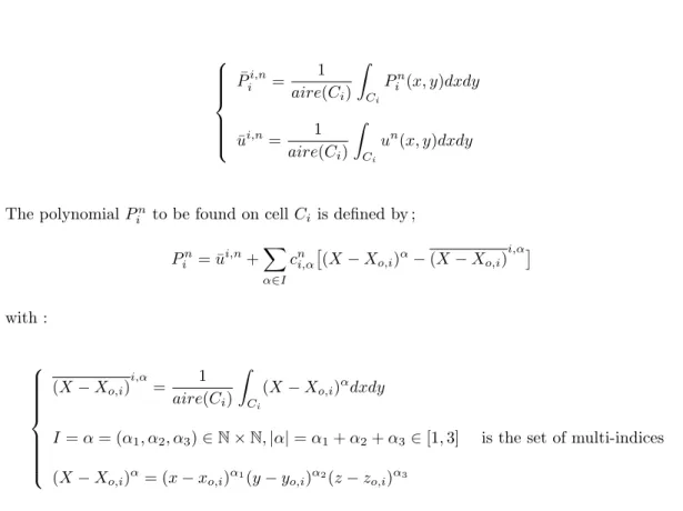
The polynomialPin to be reconstructed on the dual cellCi is defined by the following relation : Pin = ¯ui,n+X
α∈I
cni,αh
(X−Xo,i)α−(X−Xo,i)i,αi
(13) where :
(X−Xo,i)i,α=V ol(C1
i)
R
Ci(X−Xo,i)αdxdydz,
I is the set of multi-indices :I={α= (α1, α2, α3)∈N3, s.t.|α|=α1+α2+α3∈[1,2]}, (X−Xo,i)α= (x−xo,i)α1(y−yo,i)α2(z−zo,i)α3, where (xo,i, yo,i, zo,i) is the centroid ofCi. We order the multi-indices as follows :
α= 1→(α1= 1, α2= 0, α3= 0) α= 2→(α1= 0, α2= 1, α3= 0) α= 3→(α1= 0, α2= 0, α3= 1) α= 4→(α1= 1, α2= 1, α3= 0) α= 5→(α1= 1, α2= 0, α3= 1) α= 6→(α1= 0, α2= 1, α3= 1) α= 7→(α1= 2, α2= 0, α3= 0) α= 8→(α1= 0, α2= 2, α3= 0) α= 9→(α1= 0, α2= 0, α3= 2)
To build the polynomialPin on the cell Ci, we need to define the moleculeMi formed from the neighboring cells of Ci, so as to take enough values of the solution around ito reconstruct the coefficients of the polynomial. In the present case we need to calculate the 9 coefficients of the polynomial, so our molecule Mi must contain at least 9 cells (in addition toCi).
The 9 unknown coefficientscni,αof the polynomial reconstruction are calculated by the Least Squares method, i.e. such a way that the distance L2 between the means on cells Ck, of the polynomial P¯ii,n associated with the cell Ci, and of the solution u¯k,n, be minimal for cells Ck
included in the moleculeMi.
Hi= X
Ck6=i⊂Mi
P¯ik,n−u¯k,n2
(14)
whereP¯ik,nrepresents the mean of polynomialPin in cellCk : P¯ik,n= 1
V ol(Ck) Z
Ck
Pin(x, y)dxdydz. (15)
Through the construction ofCk, we get :
Hi= X
Ck6=i⊂Mi
1 V ol(Ck)
X
T∈Ck
Z
T
Pin(x, y)dxdydz−u¯k,n
!2
(16)
RR n° 9415
whereT is a subtetrahedron.
Hi=P
Ck6=i⊂Mi
h−¯uk,n+V ol(C1
k)
P
T∈Ck
R
T
¯
ui,n+P
α∈Icni,αh
(X−Xo,i)α−V ol(C1
i)
P
T∈Ci
R
T(X−Xo,i)αdxdydzi i2
The least square minimisation ofHi with respect tocni,α(α∈I), will define the polynomialPin. It writes :
δHi
δcni,α = 0, α∈I. (17)
From this condition we deduce the following system :
2∗P
k∈V(i)Di,k,1∗Kα= 0 2∗P
k∈V(i)Di,k,2∗Kα= 0 2∗P
k∈V(i)Di,k,3∗Kα= 0 2∗P
k∈V(i)Di,k,4∗Kα= 0 2∗P
k∈V(i)Di,k,5∗Kα= 0 2∗P
k∈V(i)Di,k,6∗Kα= 0 2∗P
k∈V(i)Di,k,7∗Kα= 0 2∗P
k∈V(i)Di,k,8∗Kα= 0 2∗P
k∈V(i)Di,k,9∗Kα= 0 where
Di,k,p= 1 aire(Ck)
X
T∈Ck
Z
T
(X−Xo,i)pdxdydz− 1 aire(Ci)
X
T∈Ci
Z
T
(X−Xo,i)pdxdydz forp∈[1,2,3,4,5,6,7,8,9], and :
Kα= 1 V ol(Ck)
X
T∈Ck
Z
T
¯
ui,n+X
α∈I
cni,α
"
(X−Xo,i)α− 1 V ol(Ci)
X
T∈Ci
Z
T
(X−Xo,i)αdxdydz
#!
−¯uk,n We simplifyKαby using the following relation :
1 V ol(Ck)
Z
Ck
1 V ol(Ci)
Z
Ci
un(x, y)
= ¯ui,n(x, y).
We then obtain : Kα= ¯ui,n+ 1
V ol(Ck) X
T∈Ck
Z
T
X
α∈I
cni,α(X−Xo,i)α− 1 V ol(Ci)
X
T∈Ci
Z
T
X
α∈I
cni,α(X−Xo,i)αdxdydz−¯uk,n Taking, for example the computation ofP
k∈V(i)Di,k,1∗Kα= 0, we get : X
Ck6=i⊂Mi
Di,k,1
¯ ui,n
+ X
Ck6=i⊂Mi
Di,k,1
"
1 V ol(Ck)
X
T∈Ck
Z
T
X
α∈I
cni,α(X−Xo,i)α
#
− X
Ck6=i⊂Mi
Di,k,1
"
1 V ol(Ci)
X
T∈Ci
Z
T
X
α∈I
cni,α(X−Xo,i)αdxdydz
#
− X
Ck6=i⊂Mi
Di,k,1
¯ uk,n
= 0
or in a more compact and readable manner : X
α∈I
X
Ck6=i⊂Mi
Di,k,1
1 V ol(Ck)
Z
Ck
(X−Xo,i)α− 1 V ol(Ci)
Z
Ci
(X−Xo,i)αdxdydz
cni,α
X
q∈[1,..,9]
X
Ck6=i⊂Mi
Di,k,1∗Di,k,q= X
Ck6=i⊂Mi
Di,k,1
¯
uk,n−u¯i,n X
q∈[1,..,9]
X
Ck6=i⊂Mi
Di,k,2∗Di,k,q= X
Ck6=i⊂Mi
Di,k,2
u¯k,n−u¯i,n X
q∈[1,..,9]
X
Ck6=i⊂Mi
Di,k,3∗Di,k,q= X
Ck6=i⊂Mi
Di,k,3
¯
uk,n−u¯i,n X
q∈[1,..,9]
X
Ck6=i⊂Mi
Di,k,4∗Di,k,q= X
Ck6=i⊂Mi
Di,k,4
¯
uk,n−u¯i,n X
q∈[1,..,9]
X
Ck6=i⊂Mi
Di,k,5∗Di,k,q= X
Ck6=i⊂Mi
Di,k,5
u¯k,n−u¯i,n X
q∈[1,..,9]
X
Ck6=i⊂Mi
Di,k,6∗Di,k,q= X
Ck6=i⊂Mi
Di,k,6
¯
uk,n−u¯i,n X
q∈[1,..,9]
X
Ck6=i⊂Mi
Di,k,7∗Di,k,q= X
Ck6=i⊂Mi
Di,k,7
¯
uk,n−u¯i,n X
q∈[1,..,9]
X
Ck6=i⊂Mi
Di,k,8∗Di,k,q= X
Ck6=i⊂Mi
Di,k,8
u¯k,n−u¯i,n X
q∈[1,..,9]
X
Ck6=i⊂Mi
Di,k,9∗Di,k,q= X
Ck6=i⊂Mi
Di,k,9
¯
uk,n−u¯i,n We can now re-write the least square system to solve : under a compact form :
Aicni =bni. The integrals Z
T
(X−Xo,i)αdxdydz forming the matrix are numerically computed with Gauss quadrature.
5.2 Cubic polynomial reconstruction
5.2.1 General case
On any cell Ci and any time phase we have to approximate the solution u(x, y, z, tn) = u(x, y, z)n by reconstructing it with a cunic polynomialPin.
We impose that the mean of the polynomialPin (also writtenP¯ii,n) in cellCi is exactly equal to the mean of the current solution,u¯i,n) on cellCi.
This condition is written :P¯ii,n= ¯ui,n, with :
RR n° 9415
P¯ii,n= 1 aire(Ci)
Z
Ci
Pin(x, y)dxdy
¯
ui,n= 1 aire(Ci)
Z
Ci
un(x, y)dxdy
The polynomialPin to be found on cellCi is defined by ; Pin= ¯ui,n+X
α∈I
cni,α
(X−Xo,i)α−(X−Xo,i)i,α with :
(X−Xo,i)i,α= 1 aire(Ci)
Z
Ci
(X−Xo,i)αdxdy
I=α= (α1, α2, α3)∈N×N,|α|=α1+α2+α3∈[1,3] is the set of multi-indices (X−Xo,i)α= (x−xo,i)α1(y−yo,i)α2(z−zo,i)α3
where(xo,i, yo,i, zo,i)will be taken equal to the centroid of celli.
For a degree three polynomial the coefficientsci,αare19(constant term not included).
To constructPinon cellCi, we need to define a stencilSi made of asufficiently large number of cellsneighboringCi.
Of course the stencil assembly is influenced by the number of direct neighbors. While all direct neighbors are put inSi, we need extra cells (see figure 4), and the cardinal ofSi can be as high as100in order to have an accurate reconstruction.
Figure 4 – Construction de la moléculeSi centrée au nœudi. À gauche : cas où i a au plus cinq voisins, à droite : cas oùia moins de cinq voisins.
The19unknown coefficientscni,αare again computed through a least square fitting, minimising thel2 distance between polynomial means and solution means :
Hi(cn) = X
k∈V(i)
P¯ik,n−u¯k,n2
,
whereP¯ik,nis the mean ofPin onCk : P¯ik,n= 1
aire(Ck) Z
Ck
Pin(x, y, dz)dxdydz.
Remark :In order to make easier the fitting, we can add a diagonal term as follows : Hi(cn) = X
k∈V(i)
P¯ik,n−u¯k,n2
+ εX
α
c2i,α. (18)
By construction ofCk, we can write : Hi= X
k∈V(i)
1 aire(Ck)
X
T∈Ck
Z
T
Pin(x, y, z)dxdydz−¯uk,n 2
, whereT are thesubtetrahedra of cellCk. Equivalently we have :
Hi= X
k∈V(i)
"
Hi,k
#2
; Hi,k= 1 aire(Ck)
X
T∈Ck
Z
T
−u¯k,n+ ¯ui,n+X
α∈I
cni,α
(X−Xo,i)α− 1 aire(Ci)
X
T0∈Ci
Z
T0
(X−Xo,i)αdx0dy0dz0
dxdydz Thus :
Hi= X
k∈V(i)
"
Hi,k1 +Hi,k2 +Hi,k3 +Hi,k4
#2
Hi,k1 = 1 aire(Ck)
X
T∈Ck
Z
T
(−¯uk,n)dxdydz Hi,k2 = 1
aire(Ck) X
T∈Ck
Z
T
(+¯ui,n)dxdydz Hi,k3 = 1
aire(Ck) X
T∈Ck
Z
T
X
α∈I
cni,α(X−Xo,i)α
dxdydz Hi,k4 = 1
aire(Ck) X
T∈Ck
Z
T
−X
α∈I
cni,α 1 aire(Ci)
X
T0∈Ci
Z
T0
(X−Xo,i)αdx0dy0dz0
dxdydz.
We observe that the integral on subtetraha=edra commute with the uniform functions : Hi,k1 = 1
aire(Ck) X
T∈Ck
Z
T
(−¯uk,n)dxdydz=−¯uk,n
Hi,k2 = 1 aire(Ck)
X
T∈Ck
Z
T
¯
ui,ndxdydz= ¯ui,n We have also a constant quantity :
Hi,k4 = 1 aire(Ck)
X
T∈Ck
Z
T0
X
α∈I
−cni,α
"
1 aire(Ci)
X
T0∈Ci
Z
T
(X−Xo,i)αdx0dy0dz0
#
dxdydz=
X
α∈I
−cni,α 1
aire(Ci) X
T0∈Ci
Z
T0
(X−Xo,i)αdx0dy0dz0
#
= X
α∈I
−cni,α
Di,α
aire(Ci)
#
RR n° 9415
whre we have introduced the notation : Di,α= X
T∈Ci
Z
T
(X−Xo,i)αdxdydz.
Implementation :
DO igauss = 1,4 DO m = 1,3
cg(m) = (alp1(igauss)-1.0)*c(m,i)
1 + alp2(igauss)*cIij(m)
1 + alp3(igauss)*cgijk(m)
1 + alp4(igauss)*cGijkl(m)
ENDDO ! DO m = 1,3
c Contributions to integrals of 1, x,x*x,x*y,x*z c Contributions to integrals of 1, y,y*x,y*y,y*z c Contributions to integrals of 1, z,z*x,z*y,z*z
sum0 = sum0 + wgtval(igauss)*volminitet sum(is) = sum(is) + wgtval(igauss)*volminitet sumx(is) = sumx(is) + cg(1)*wgtval(igauss)*volminitet sumy(is) = sumy(is) + cg(2)*wgtval(igauss)*volminitet sumz(is) = sumz(is) + cg(3)*wgtval(igauss)*volminitet
sumxx(is) = sumxx(is) + cg(1)*cg(1)*wgtval(igauss)*volminitet sumyx(is) = sumyx(is) + cg(2)*cg(1)*wgtval(igauss)*volminitet sumzx(is) = sumzx(is) + cg(3)*cg(1)*wgtval(igauss)*volminitet sumyy(is) = sumyy(is) + cg(2)*cg(2)*wgtval(igauss)*volminitet sumzy(is) = sumzy(is) + cg(3)*cg(2)*wgtval(igauss)*volminitet sumzz(is) = sumzz(is) + cg(3)*cg(3)*wgtval(igauss)*volminitet ENDDO ! DO igauss = 1,4
We also introduce the following notations : D¯i,k,α= 1
aire(Ck) X
T∈Ck
Z
T
(X−Xo,i)αdxdydz and :
Di,k,α= ¯Di,k,α− Di,α
aire(Ci). Finally we have shown that :
Hi,k =Hi,k1 +Hi,k2 +Hi,k3 +Hi,k4 with :
Hi,k1 =−¯uk,n
Hi,k2 = ¯ui,n Hi,k3 = 1
aire(Ck) X
T∈Ck
Z
T
X
α∈I
cni,α(X−Xo,i)α
dxdydz=X
α∈I
cni,αD¯i,k,α
Hi,k4 =X
α∈I
−cni,α
Di,α
aire(Ci)
# . We deduce a simplified writting forHi,k :
Hi,k=−¯uk,n+ ¯ui,n+X
α∈I
cni,α
"
+ ¯Di,k,α− Di,α
aire(Ci)
#
= −¯uk,n+ ¯ui,n+X
α∈I
cni,αDi,k,α. We transform now the numbering of monomials in a more tractable form :
1≤ |αp| ≤3⇔αp∈ {α1, α2, α3, α4, α5, α6, α7, α8, α9, α10, α10, α11, α12, α13, α14, α15, α16, α17, α18, α19,} (19)
Dα1 =Dx, Dα2 =Dy, Dα3 =Dz, Dα4 =Dxx, , Dα5 =Dyy, Dα6=Dzz,
Dα7=Dxy, Dα8 =Dxz, Dα9 =Dyz, Dα10 =Dxxx, Dα11 =Dyyy, Dα12 =Dzzz, Dα13 =Dxxy, Dα14 =Dxxz,
Dα15 =Dxyy, Dα16 =Dyyz, Dα17 =Dxzz, Dα18 =Dyzz, Dα19=Dxyz, (20)
with the adapted notation :
Di,p=Di,αp ; D¯i,k,p= ¯Di,k,αp ; Di,k,p=Di,k,αp
Let us transformthe terms P
T∈Ck
R
T(X−Xo,i)α dxdydz présents dans D¯i,k,α. We remark that (forα1= (1,0,0))
X
T∈Ck
Z
T
(x−x(i))dxdydz= X
T∈Ck
Z
T
(x−x(k))dxdydz+aire(Ck)(x(k)−x(i))
(21) which implies that
Di,k,1= Dk,1
aire(Ck)+ (x(k)−x(i))− Di,1
aire(Ci) Di,k,2= Dk,2
aire(Ck)+ (y(k)−y(i))− Di,2 aire(Ci) Di,k,3= Dk,3
aire(Ck)+ (z(k)−z(i))− Di,3
aire(Ci).
(22)
RR n° 9415
x = coco(1,is) y = coco(2,is) z = coco(3,is) xsv = coco(1,isv) ysv = coco(2,isv) zsv = coco(3,isv) dxsv = x - xsv dysv = y - ysv dzsv = z - zsv
DD(ineig,1) = D(1,2)/vols(isv) - dxsv - D(1,1)/vols(is) DD(ineig,2) = D(2,2)/vols(isv) - dysv - D(2,1)/vols(is) DD(ineig,3) = D(3,2)/vols(isv) - dzsv - D(3,1)/vols(is) Remarking that :
(x−x(i))2 = x2−2x(i)x+x(i)2
= x2−2x(k)x+x(k)2−2x(i)x+ 2x(k)x+x(i)2−x(k)2
= x2−2x(k)x+x(k)2−2(x(i)−x(k))x+ (x(i)2−x(k)2)
(x−x(i))2 = (x−x(k))2−2(x(i)−x(k))(x−x(k))−2(x(i)−x(k))x(k) + (x(i)2−x(k)2)
= (x−x(k))2−2(x(i)−x(k))(x−x(k))−2(x(i)−x(k))x(k) + (x(i)2−x(k)2)
= (x−x(k))2−2(x(i)−x(k))(x−x(k)) +x(i)2−2x(i)x(k) +x(k)2
= (x−x(k))2−2(x(i)−x(k))(x−x(k)) +x(i)2−2x(i)x(k) +x(k)2
= (x−x(k))2−2(x(i)−x(k))(x−x(k)) + (x(i)−x(k))2 We deduce :
X
T∈Ck
Z
T
(x−x(i))2dxdydz= X
T∈Ck
Z
T
(x−x(k))2dxdydz
−2(x(i)−x(k)) X
T∈Ck
Z
T
(x−x(k))dxdydz +aire(Ck)(x(i)−x(k))2
(23) which also writes (α4= (2,0,0,), α1= (1,0,0,):
X
T∈Ck
Z
T
(x−x(i))2dxdydz=Dk,4−2(x(i)−x(k))Dk,1+aire(Ck)(x(i)−x(k))2.
(24) De même en y :
X
T∈Ck
Z
T
(y−y(i))2dxdydz=Dk,5−2(y(i)−y(k))Dk,2+aire(Ck)(y(i)−y(k))2.
(25)
Similarly inz :
X
T∈Ck
Z
T
(z−z(i))2dxdydz=Dk,6−2(z(i)−z(k))Dk,3+aire(Ck)(z(i)−z(k))2.
(26)
Which also writes :
Di,k,4= Dk,4−2(x(i)−x(k))Dk,1
aire(Ck) + (x(i)−x(k))2− Di,4
aire(Ci). Di,k,5=Dk,5−2(y(i)−y(k))Dk,2
aire(Ck) + (y(i)−y(k))2− Di,5
aire(Ci). Di,k,6= Dk,6−2(z(i)−z(k))Dk,3
aire(Ck) + (z(i)−z(k))2− Di,6 aire(Ci).
(27)
DD(ineig,4) = ( D(4,2)-2*dxsv*D(1,2) )/vols(isv) + dxsv**2 - D(4,1)/vols(is) DD(ineig,5) = ( D(5,2)-2*dysv*D(2,2) )/vols(isv) + dysv**2 - D(5,1)/vols(is) DD(ineig,6) = ( D(6,2)-2*dzsv*D(3,2) )/vols(isv) + dzsv**2 - D(6,1)/vols(is)
Remarking that :
(x−x(i))(y−y(i)) = (x−x(k))(y−y(k)) + (x−x(i))(y−y(i))−(x−x(k))(y−y(k))
= (x−x(k))(y−y(k))−(x(i)−x(k))y
−(y(i)−y(k))x+x(i)y(i)−x(k)y(k)
= (x−x(k))(y−y(k))
−(x(i)−x(k))(y−y(k))−(x(i)−x(k)y(k)
−(y(i)−y(k))(x−x(k))−(y(i)−y(k))x(k) +x(i)y(i)−x(k)y(k)
= (x−x(k))(y−y(k))−(x(i)−x(k))(y−y(k))−(y(i)−y(k))(x−x(k))
−x(i)y(k) +x(k)y(k)−y(i)x(k) +y(k))x(k) +x(i)y(i)−x(k)y(k)
= (x−x(k))(y−y(k))−(x(i)−x(k))(y−y(k))−(y(i)−y(k))(x−x(k))
−x(i)y(k) +x(k)y(k)−y(i)x(k) +x(i)y(i)
RR n° 9415
We derive :
Di,k,7 = Dk,7−(x(i)−x(k))Dk,2−(y(i)−y(k))Dk,1 aire(Ck)
+x(i)y(i) +x(k)y(k)−x(i)y(k)−x(k)y(i)− Di,7
aire(Ci) Di,k,8 = Dk,8−(x(i)−x(k))Dk,3−(z(i)−z(k))Dk,1
aire(Ck)
+x(i)z(i) +x(k)z(k)−x(i)z(k)−x(k)z(i)− Di,8 aire(Ci) Di,k,9 = Dk,9−(y(i)−y(k))Dk,3−(z(i)−z(k))Dk,2
aire(Ck)
+y(i)z(i) +y(k)z(k)−y(i)z(k)−y(k)z(i)− Di,9
aire(Ci).
(28) DD(ineig,7) = ( D(7,2)-dxsv*D(2,2) - dysv*D(1,2) )/vols(isv)
DD(ineig,8) = ( D(8,2)-dxsv*D(3,2) - dzsv*D(1,2) )/vols(isv) DD(ineig,9) = ( D(9,2)-dysv*D(3,2) - dzsv*D(2,2) )/vols(isv)
DD(ineig,7) = DD(ineig,7) + (y*y-xsv*ysv-x*ysv-xsv*y) - D(7,1) /vols(is) DD(ineig,8) = DD(ineig,8) + (x*z-xsv*zsv-x*zsv-xsv*z) - D(8,1) /vols(is) DD(ineig,9) = DD(ineig,9) + (y*z-ysv*zsv-y*zsv-ysv*z) - D(9,1) /vols(is) Remarking that :
(x−x(i))3= (x−x(k)−x(i) +x(k))3
Puttinga= (x−x(k)), b= (x(i)−x(k))and using the fact that :(a−b)3= a3−3a2b+ 3ab2−b3, we have :(x−x(i))3=
(x−x(k))3−3(x−x(k))2(x(i)−x(k)) + 3(x−x(k))(x(i)−x(k))2−(x(i)−x(k))3 Putting(x(i)−x(k)) =dx,(y(i)−y(k)) =dy,(z(i)−z(k)) =dzwe deduce :
Di,k,10 = 3dx2Dk,1−3dxDk,4+Dk,10
aire(Ck) −dx3− Di,10
aire(Ci) Di,k,11 = 3dy2Dk,2−3dyDk,5+Dk,11
aire(Ck) −dy3− Di,11
aire(Ci) Di,k,12 = 3dz2Dk,3−3dzDk,6+Dk,12
aire(Ck) −dz3− Di,12
aire(Ci)
(29) Remarking that :
(x−x(i))(y−y(i))2= (x−x(k)−x(i) +x(k))(y−y(k)−y(i) +y(k))2
puttinga= (x−x(k)),b = (x(i)−x(k)), c= (y−y(k)), d= (y(i)−y(k))and using the fact that :(a−b)(c−d)2=
ac2−2acd+ad2−bc2+ 2bcd−bd2, we have :(x−x(i))(y−y(i))2= (x−x(k))(y−y(k))2−2(x−x(k))(y−y(k))(y(i)−y(k))
+ (x−x(k))(y(i)−y(k))2−(x(i)−x(k))(y−y(k))2
+ 2(x(i)−x(k))(y−y(k))(y(i)−y(k))−(x(i)−x(k)(y(i)−y(k))2
Putting(x(i)−x(k)) =dx,(y(i)−y(k)) =dy,(z(i)−z(k)) =dz we deduce : Di,k,13 = dx2Dk,2+ 2dxdyDk,1−2dxDk,7−dyDk,4+Dk,13
aire(Ck) −dx2dy− Di,13
aire(Ci) Di,k,14 = dx2Dk,3+ 2dxdzDk,1−2dxDk,8−dzDk,4+Dk,14
aire(Ck) −dx2dz− Di,14
aire(Ci) Di,k,15 = dy2Dk,1+ 2dxdyDk,2−2dyDk,7−dxDk,5+Dk,15
aire(Ck) −dy2dx− Di,15
aire(Ci) Di,k,16 = dy2Dk,3+ 2dzdyDk,2−2dyDk,9−dzDk,5+Dk,16
aire(Ck) −dy2dz− Di,16
aire(Ci) Di,k,17 = dz2Dk,1+ 2dxdzDk,3−2dzDk,8−dxDk,6+Dk,17
aire(Ck) −dz2dx− Di,17 aire(Ci) Di,k,18 = dz2Dk,2+ 2dydzDk,3−2dzDk,9−dyDk,6+Dk,18
aire(Ck) −dz2dy− Di,18
aire(Ci) (30) Remarking that :
(x−x(i))(y−y(i))(z−z(i)) = (x−x(k)−x(i) +x(k))(y−y(k)−y(i) +y(k))(z−z(k)−z(i) +z(k)) putting a= (x−x(k)),b= (x(i)−x(k)), c= (y−y(k)),d= (y(i)−y(k)),e= (z−z(k)),f = (z(i)−z(k))and using that :(a−b)(c−d)(e−f) =
eac−ead−ebc+ebd−f ac+f ad+f bc−f bd, we get :(x−x(i))(y−y(i))(z−z(i)) = (z− z(k))(x−x(k))(y−y(k))
−(z−z(k))(x−x(k))(y(i)−y(k))
−(z−z(k))(x(i)−x(k))(y−y(k)) + (z−z(k))(x(i)−x(k))(y(i)−y(k))
−(z(i)−z(k))(x−x(k))(y−y(k)) + (z(i)−z(k))(x−x(k))(y(i)−y(k)) + (z(i)−z(k))(x(i)−x(k))(y−y(k))
−(z(i)−z(k))(x(i)−x(k))(y(i)−y(k))
Putting(x(i)−x(k)) =dx,(y(i)−y(k)) =dy,(z(i)−z(k)) =dz we deduce :
Di,k,19 = −dxDk,9−dyDk,8−dzDk,7+dydzDk,1+dxdzDk,2+dxdyDk,3+Dk,19
aire(Ck)
−dxdydz− Di,19
aire(Ci)
(31) 5.2.2 Partition case
Over each molecule we reconstruct only one polynomial PMi using the previous technique over the most centered cell in the molecule. Defined by
Crep=argminCi∈M i|cg(Ci)−cg(Mi)| (32)
RR n° 9415
Where cg() is the center of gravity.
Once the polynomials coefficients are obtained we have to add a constant therm Pk0 in order to obtain :
1 Ck
Z
Ck
PMi+Pk0= ¯uk,n,∀Ck∈Mi (33) Using the polynomial definition we have :
1 Ck
Z
Ck
PMi= 1 Ck
Z
Ck
¯
urep,n+X
α∈I
cnrep,α
(X−Xo,rep)α−(X−Xo,rep)rep,α
(34)
= ¯urep,n+X
α∈I
cnrep,α 1 Ck
Z
Ck
(X−Xo,rep)α−(X−Xo,rep)rep,α (35)
= ¯urep,n+X
α∈I
cnrep,αD¯rep,k,α− 1
aire(Crep)Drep,α (36)
= ¯urep,n+X
α∈I
cnrep,α
Drep,k,α
(37)
Then the constants terms are defined as :
Pk0= ¯uk,n−u¯rep,n−X
α∈I
cnrep,α
Drep,k,α (38)
6 Flux evaluation
6.1 Flux evaluation for third-order accuracy
The next objective is to evaluate the flow at timeton the interfaces between the cellCiand its neighborsCk. We use a 3-point Gaussian quadrature on the external facets of the sub-tetrahedra.
Recall that the flow on the border of a cell can be written : Z
∂Ci
f(u(x, y, t))·nds= X
k inV(i)
Z
∂Ci∩∂Ck
f(u(x, y, t))·nds
The intersection between two cells ∂Ci ∩∂Ck can be broken down into several triangles as shown in Figure 5. We arbitrarily number these trianglesT{i,k,r}, with1≤r≤Ri,k, whereRi,k
represents the total number of triangle making up the interface∂Ci∩∂Ck. Z
∂Ci
f(u(x, y, t))·nds= X
k∈V(i)
X
1≤r≤Ri,k,
Z
T{i,k,r}
f(u(x, y, t))·nds.
On the whole cell Ci, the solution u(x, y, z) is approximated by the polynomial Pin defined in previous section.
Z
∂Ci
f(u(x, y, t))·nds= X
k∈V(i)
X
1≤r≤Ri,k,
Z
T{i,k,r}
f(Pi(x, y, z, t))·nds.
Figure5 – Numerical quadrature for flux integration.
We use a Gauss quadrature (Figure 5) with three integration nodes for the evaluation of R
T{i,k,r}f(Pi(x, y, z, t))·nds. For a triangle T{i,k,r} we denote the Gauss nodes pl{i,k,r} =
(xl{i,k,r}, y{i,k,r}l , zl{i,k,r})withl∈[1,2,3]and their weightsω= 13. Z
∂Ci
f(u(x, y, t))·nds= X
k∈V(i)
X
1≤r≤Ri,k
X
l∈[1,2,3]
ωf
Pi(pl{i,k,r}, t)
·n{i,k,r}ds withn{i,k,r}=R
T{i,k,r}n(x, y, z)ds.
However, since two distinct polynomials Pi and Pk were constructed on either side of the interface between cells Ci and Ck, the reconstructed solution on each Gaussian point takes two a prioridifferent values.
Therefore we approximate the flux on theT{i,k,r} interface by a numericalΦflux function : f
Pi
pl{i,k,r}, t
·n= Φ Pi
pl{i,k,r}, t , Pk
pl{i,k,r}, t
,n{i,k,r}
We need to choose the numerical fluxΦsuch that the resulting scheme is stable. We choose the Donor Cell upwind solver, defined by the following relation :
Φ (u1, u2,v) = f(u1) +f(u2)
2 ·v−γ
2
∂f
∂v
u1+u2 2
·v
(u2−u1) (39) where the regular option is to takeγ= 1..
6.2 Flux evaluation for fourth-order accuracy
We follow the recommandation in [14] who propose the integration described in Table 1 .
RR n° 9415