Un algorithme de fouille de données générique et parallèle pour architecture multi-coeurs

(1)

HAL Id: tel-00680025

https://tel.archives-ouvertes.fr/tel-00680025

Submitted on 17 Mar 2012

HAL is a multi-disciplinary open access archive for the deposit and dissemination of scientific research documents, whether they are published or not. The documents may come from teaching and research institutions in France or abroad, or from public or private research centers.

L’archive ouverte pluridisciplinaire HAL, est destinée au dépôt et à la diffusion de documents scientifiques de niveau recherche, publiés ou non, émanant des établissements d’enseignement et de recherche français ou étrangers, des laboratoires publics ou privés.

parallèle pour architecture multi-coeurs

Benjamin Negrevergne

To cite this version:

Benjamin Negrevergne. Un algorithme de fouille de données générique et parallèle pour architecture multi-coeurs. Autre [cs.OH]. Université de Grenoble, 2011. Français. �NNT : 2011GRENM062�. �tel- 00680025�

(2)

Pour obtenir le grade de

DOCTEUR DE L’UNIVERSIT ´ E DE GRENOBLE

Sp ´ecialit ´e : Informatique

Arr êt é minist ériel : 7 Ao ût 2006

Pr ´esent ´ee par

Benjamin Negrevergne

Th `ese dirig ´ee parMarie-Christine Rousset,

pr ´epar ´ee au sein du Laboratoire d’Informatique de Grenoble et de l’EDMSTII.

A Generic and Parallel Pattern Min- ing Algorithm for Multi-Core Archi- tectures

Th `ese soutenue publiquement le29 Novembre 2011, devant le jury compos ´e de :

M Jean-Franc¸ois M ´ehaut

Professeur à L’Universit é de Grenoble, Pr ésident

M Hiroki Arimura

Professeur `a l’Universit ´e d’Hokkaido, Rapporteur

M Bruno Cr ´emilleux

Professeur `a l’Universit ´e de Caen, Rapporteur

Mme Anne Laurent

Professeur `a l’Universit ´e de Montpellier, Examinatrice

Mme Marie-Christine Rousset

Professeur à L’Universit é de Grenoble, Directrice de th èse

M Alexandre Termier

Maˆıtre de conf érences à l’Universit é de Grenoble, Co-Directeur de th èse

(3)

(4)

Mots-clefs : Fouille de données, extraction de motifs fréquents, systèmes d’ensembles accessibles, algorithmes parallèles, calcul haute performance, évaluation de performances, architectures multi-cœurs.

Résumé : Dans le domaine de l’extraction de motifs, il existe un grand nombre d’algorithmes pour résoudre une large variété de sous problèmes sensiblement identiques.

Cette variété d’algorithmes freine l’adoption des techniques d’extraction de motifs pour l’analyse de données. Dans cette thèse, nous proposons un formalisme qui permet de capturer une large gamme de problèmes d’extraction de motifs. Pour démontrer la généralité de ce formalisme, nous l’utilisons pour décrire trois problèmes d’extraction de motifs : le problème d’extraction d’itemsets fréquents fermés, le problème d’extraction de graphes relationnels fermés ou le problème d’extraction d’itemsets graduels fermés.

Ce formalisme nous permet de construire ParaMinerqui est un algorithme générique et parallèle pour les problèmes d’extraction de motifs. ParaMinerest capable de résoudre tous les problèmes d’extraction de motifs qui peuvent être décrits dans notre formalisme.

Pour obtenir de bonnes performances, nous avons généralisé plusieurs optimisations pro- posées par la communauté dans le cadre de problèmes spécifiques d’extraction de motifs.

Nous avons également exploité la puissance de calcul disponible dans les architectures parallèles.

Nos expériences démontrent qu’en dépit de la généralité deParaMiner, ses performances sont comparables à celles obtenues par les algorithmes les plus rapides de l’état de l’art. Ces algorithmes bénéficient pourtant d’un avantage important, puisqu’ils incorporent de nom- breuses optimisations spécifiques au sous problème d’extraction de motifs qu’ils résolvent.

Th`ese effectu´ee au Laboratoire d’Informatique de Grenoble Laboratoire LIG - UMR 5217

Maison Jean Kuntzmann - 110 av. de la Chimie - Domaine Universitaire de Saint-Martin-d’H`eres - BP 53

38041 Grenoble cedex 9 - France

Tel. : +33 (0)4 76 51 43 61 - Fax : +33 (0)4 76 51 49 85

(5)

(6)

Keywords: Data mining, pattern mining, accessible set systems, parallel algorithms, high performance computing, performance evaluation, multi-core architectures.

Abstract: In the pattern mining field, there exists a large number of algorithms that can solve a large variety of distinct but similar pattern mining problems. This variety prevent broad adoption of data analysis with pattern mining algorithms. In this thesis we propose a formal framework that is able to capture a broad range of pattern mining problems. We illustrate the generality of our framework by formalizing three different pattern mining problems: the problem of closed frequent itemset mining, the problem of closed relational graph mining and the problem of closed gradual itemset mining.

Building on this framework, we have designed ParaMiner, a generic and parallel algorithm for pattern mining. ParaMiner is able to solve any pattern mining problem that can be formalized within our framework. In order to achieve practical efficiency we have generalized important optimizations from state of the art algorithms and we have made ParaMiner able to exploit parallel computing platforms.

We have conducted thorough experiments that demonstrate that despite being a generic algorithm, ParaMinercan compete with the fastest ad-hoc algorithms.

(7)

Remerciements

Cette thèse est le fruit du travail d’un groupe formé par ma directrice de thèse Marie- Christine Rousset, mon co-directeur de thèse Alexandre Termier, Jean-Fran¸cois Méhaut et moi même.

Merci à eux trois qui ont énormément contribué à ce travail et à mon enrichissement profes- sionnel et personnel. Particulièrement merci à Marie-Christine pour sa détermination sub- juguante, et pour le temps qu’elle m’a accordé pour corriger et mettre au point différents aspects de cette thèse. Merci à Alexandre qui à su rendre ce travail très intéressant et agréable. Au cours de cette thèse, Alexandre est resté réceptif à touts mes idées tout en sachant les canaliser pour garder mon travail cohérent et constructif. Enfin merci à Jean-Fran¸cois qui a fait preuve d’une extraordinaire patience à mon égard. Grâce à lui j’ai sans doute appris plus de choses qu’il ne le soup¸conne.

Merci à mes deux rapporteurs Hiroki Arimura et Bruno Crémilleux pour avoir bien voulu relire cette thèse, pour m’avoir prodigué des commentaires nombreux et constructifs et pour être venus assister à ma soutenance.

Pour m’avoir accueilli dans son laboratoire de Tokyo au Japon, merci au professeur Takeaki Uno. Le séjour que j’ai passé là bas a été une expérience unique et marquante que je n’oublierai pas.

Merci également à tous les membres des équipes Hadas et Mescal que j’ai côtoyés au cours de ma thèse. Tous ont eu un rôle important et méritent de faire partie de cette page de remerciements.

Certains de mes amis ont directement contribué au fond et à la forme de ma thèse. C’est le cas notamment de Judith Dehail et de Jérôme Reybert. Au delà de ces aspects techniques, Judith et Jérôme ont tous deux été des amis extraordinaires sans lesquels je ne serais pas arrivé au bout, merci à eux.

Je voudrais également remercier Rémi Tournaire, qui a eu un rôle complexe, mais indis- cutablement positif dans l’accomplissement de ce travail. Merci aussi à Christophe, Kiril et Guillaume avec qui j’ai passé des moments extraordinaires à Grenoble. Merci également

`

a Gabriel, Augustin, Aurélie et Sawako. Enfin merci à Pierre de m’avoir écouté patiem- ment me plaindre de plus en plus fréquemment au fur et à mesure que la fin de ma thèse approchait.

Merci à mon formidable ami d’enfance Brice et à tous nos amis communs : Sébastien, Mag, David, Julien, Thomas et Emie.

Enfin, merci à tous les membres de ma famille, à mon frère Camille pour m’avoir donné le goût des disciplines scientifiques, à ma sœur Marie pour son énergie et sa motivation sans limite. Et merci à mes parents Catherine et Michel pour leur soutien discret mais palpable.

Cette thèse est dédiée à mes filleuls Quentin et Charlie.

v

(8)

Chapter 1 Introduction

In 1994, Agrawal and Srikant took the list of the sale records of a retail store and tried to discover knowledge about buying habits of customers. They did so by extracting recurring patterns from the list of receipts. These patterns consisted in sets of items frequently occurring together in customer baskets. For example the pattern {cereals, milk} is likely to be a frequent one since most people buy milk with their cereals.

The frequent sets of items and their frequency can later be turned into association rules in order to know whether customers who bought milk are likely to buy cereals, or the opposite. In this context, the association rule: cereals → milk – stating that people buying cereals are likely to buy milk – is the most likely one. The association rules extracted from a retail store dataset are considered as valuable knowledge to rearrange items in shelfs and improve sales.

Back then Agrawal’s work on pattern mining was pushed by the progress in bar-code technology and the increasing data storage capacities. Nowadays, recording devices are ubiquitous and almost every piece of information is digitally recorded. In the scientific field, collecting tremendous amounts of experimental data has become a standard. At the CERN in Geneva, the Large Hadron Collider produces over 15 million gigabytes of experimental data every year. Other scientific applications in chemistry, meteorology and micro biology generate similar amounts of data.

For centuries, results of scientific experiments were carefully analyzed by experts with strong knowledge in the field. However, no human beings are capable of tackling the tremendous amounts of data generated by modern scientific experiments. Hence computer programs are now required to assist the domain experts to analyze their experimental data.

These programs can help to discover relevant informations from an ocean of mostly noisy data.

Since 1994, the pattern mining community has grown and gain in diversity. It is today an important topic of computer science addressed by many scientific publications in in- ternational conferences. In order to harness the diversity of the pattern mining problems, researchers have proposed various techniques that fall into two categories: the statistical approach and the structural approach.

The traditional approach to handle large amounts of data is to use statistics. Nowadays, 1

(11)

statistical approaches for pattern mining are widely used to mine for knowledge in very large graphs such as the web, social networks or even gene networks. In this context, so called statistical graph mining algorithms are used to compute general informations such as statistical distributions of the node degrees or such as typical topologies of small clusters[KTF09, MN08]. This approach allows to infer global properties about the input graph and spot representative or dissimilar patterns in this graph. Statistical approaches can tackle very large input datasets and provide informative knowledge over the dataset.

The other approach is in the direct vein of Agrawal’s pattern mining algorithm. It consists in extracting algebraic substructures such as sets but also sequences or graphs from the input dataset. Relevant substructures are identified according to whatever property is meaningful to the application. In most applications the frequency of a pattern is the basic property to discriminate irrelevant patterns, but not always. In this thesis we exclusively deal with this approach of pattern mining so called structural pattern mining.

1.1 Structural pattern mining

Pushed by the interesting results obtained in the context of market basket analysis, experts from other scientific domains with large set of experimental data, started to show interest in pattern mining techniques. In collaboration with researchers from the pattern mining community, they have elaborated new algorithms to extract meaningful patterns from their datasets.

O O

O

O O O

N N

N

+

N

-

H H H

H H H H

H H

H H H

H H

H

H H

H H H

H H

H H H H

H

H H

Br

O O

O O O

N N

N N+

N-

H H H

H H

H

H H H

H

(a) anti-HIV active molecule 1 (b) anti-HIV active molecule 2

O O O O

N N

N

+

N

-

H H H

H H

H H H H

H

H H

(c) anti-HIV molecular pattern

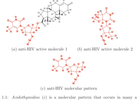
Figure 1.1: Azidothymidine (c) is a molecular pattern that occurs in many anti-HIV molecules such as (a) and (b).

For example, chemical engineers were interested in extracting characteristic substructures from datasets of chemical compounds. In [KDRH01] Kramer et al. have mined a dataset of molecules represented as graphs. Those molecules had been previously tested for their capability to protect human cells from the HIV infection (an example of such molecules

(12)

Date Temp. ( C) Pressure (hPa) Wind direction Wind speed (km/h)

May 26 2011 17.6 1021.20 300 57

May 27 2011 18.5 1021.30 310 57

May 28 2011 20.4 1018.20 320 51

May 29 2011 28.5 1012.80 110 26

May 30 2011 18.9 1014.80 290 67

May 31 2011 16.5 1026.50 310 77

Figure 1.2: Meteorological records of climate taken from May 25 2011 to May 31 2011, at 6pm, in France. The gradual pattern {T ↑, P ↓, W ind↑}is observable day 26, 28, 29 and 31.

is shown in figure 1.1 (a) and (b)). The goal was to extract the substructures commonly occurring in anti-HIV molecules (e.g. figure 1.1 (c)). Although in [KDRH01] Kramer et al.

were only able to extract linear fragments of this compound, other approaches developed by Inokuchi et al. in [IWM00] and Yan et al. in [YH02] are capable of extracting full graph patterns such as in figure 1.1 (c). Graph mining is a useful application to analyze many other types of dataset such as web logs or gene networks datasets.

Yet some datasets were still out of reach. Recently in [DJLT09], Di-Jorio et al have conducted work in order to analyze datasets consisting in large amounts of quantitative data. The goal is to extract correlated variations of quantitative values. For example, the dataset in figure 1.2 is a list of records from various climatic sensors. Given this dataset, one may want to know if there exists any correlation between the measured values. A fine analysis of this dataset reveals that in 67% of the records, when the temperature increases the pressure decreases and the wind speed increases. Gradual pattern mining is able to extract such co-variations formalized as {T ↑, P ↓, W ind↑}. Di-Jorio in[DJLT09]

have worked on gradual pattern mining in order to extract co-variations in datasets with hundreds of attributes and thousands of records. This type of pattern is helpful to mine survey database, data streams or network sensors readings.

Because of the diversity of the datasets and the patterns to extract, most people having interest in pattern mining have developed their own ad-hoc algorithm adapted to their needs. Although the problems addressed by those algorithms look quite different, they are all different instances of the same problem: structural pattern mining. In this thesis, we define the problem of structural pattern mining as follows:

Given a dataset, a patternstructure definitionand a patternselection criterion, extract the set of patterns made up of all the structures occurring in the dataset satisfying the selection criterion.

The datasetis the input data to mine. In the context of basket market analysis, the dataset is a list of receipts where each receipt is a set of items purchased together. It can also be a set of molecules, when mining for substructures in chemical compounds, or the list of records from climatic sensors when mining for gradual patterns.

The pattern structure definitionspecifies the structure of the patterns to extract. It is set according to dataset structure and the application needs. For example, in the context of market basket analysis, patterns are subsets of the set of available items.

When mining molecular compounds, the patterns are labeled graphs where vertices

(13)

are labeled with chemical elements names in a given set and edges are labeled with covalent bound types. The pattern structure definition intentionally defines the set of all the candidate patterns.

Thepattern selection criterionis formulated by the application experts. A candidate pattern must meet this criterion in order to be an actual pattern. It discriminates patterns relevant to the application from irrelevant ones. The frequency is commonly used to discard irrelevant patterns, however it can be combined with other requirements such as the pattern must be a connected graph (see. Section 2.2.2).

When it’s clear from context, pattern mining will be used as a shortcut for structural pattern mining.

Pattern mining is a very difficult problem that raises many important challenges such as:

Encoding and preprocessing of raw data.

Handling the combinatorial explosion of the number of candidate patterns.

Filtering and analyzing patterns that are extracted.

In this thesis we address the second challenge by generalizing in a principled way several optimizations and by incorporating them into a generic and parallel pattern mining algorithm.

1.2 Scope of this thesis

The standard method to output the set of patterns is to generatecandidate patterns with respect to the pattern structure definition, and then test if they occur in the dataset and satisfy the selection criterion. However the number of candidate patterns to test is theoretically tremendous. For example if a retail store, selling 1000 distinct items, wants to mine its sale records to extract frequent sets of items, the number of candidate patterns is as big as 2¹⁰⁰⁰(∼10³⁰⁰). Generating and testing this amount of candidate patterns is not feasible in practice.

To reduce the number of candidate patterns and simplify the process of testing them, most pattern mining algorithms were designed to take advantage of the specificities of patterns and datasets to mine.

In [AS94], Agrawal and Srikant address the problem of mining frequent subsets by exploiting the anti-monotonicity property of the frequent sets. This property states that any set including an infrequent subset is also infrequent. Based on this property, Agrawal’s algorithm avoids generating all the candidate patterns including one or more infrequent subset. This principle was later adapted to mine other types of frequent patterns such as frequent graphs in [IWM00].

In [HPY00], Han et al. have proposed^FP-growth, a depth-first-search recursive algorithm which starts from a frequent set and efficiently computes the frequent supersets of this set.

InFP-growthitems occurring in the dataset are stored in a prefix tree like structure called FP-tree. ^FP-growthavoids costly database scans by building for each recursive call a new FP-tree representing only the sub-dataset relevant to the recursive call being processed.

(14)

Since larger frequent sets are less represented in the dataset, FP-trees get smaller as the algorithm gets deeper in the recursive calls. This approach allowed^FP-growth to tackle big datasets with a divide and conquer approach. An improved version of this technique is used in the fastest frequent set mining algorithms, LCM[UKA04].

Reducing the number of candidate patterns may not be sufficient to tackle large datasets because the number of patterns can be large as well. In order to avoid the combinatorial explosion of the number of patterns, recent algorithms focus on the extraction of closed patterns only. Closed patterns were introduced by Pasquier et al. in [PBTL99] in the context of mining frequent sets. A frequent set is closed if and only if there exist no strict supersets occurring in the dataset with an equal frequency. Mining closed frequent sets represents no loss of information over mining frequent sets. It is indeed possible to derive the identity and the frequency of any frequent set from the set of closed sets. It is also more concise; in practice the number of closed frequent sets can be orders of magnitude smaller than the number of frequent sets. Closed pattern mining is a major issue to reach efficiency in pattern mining, thus various types of closure operator were defined for other types of patterns such as trees, graphs and even gradual patterns.

In order to tackle bigger datasets researchers have worked on pattern mining algorithms able to exploit parallel architectures. The problem has attracted more attention since the parallelism became truly ubiquitous with the advent of multi-core architectures. In- deed, almost every processor available nowadays embeds two or more computing cores providing true parallelism at low cost. However naive parallelizations of pattern mining algorithms perform poorly on multi-core platforms due to load imbalance or excessive memory consumption. The problem of designing pattern mining algorithms for multi-core architectures has been addressed by several research papers in the context of frequent set mining [LOP07, NTMU10], tree mining [TP09] or graph mining [BPC06]. These papers have shown that dynamic work distribution strategies and customized data structures can reduce the load imbalance and the memory consumption. Both are required to achieve good scalability with the number of cores used to run the algorithm.

The additional computational power available in multi-core architectures, together with the algorithmic improvements mentioned above, should allow to tackle many real world datasets. However, very few pattern mining algorithms fully integrate these research works. Indeed, the lack of an unified definition for pattern mining problems make any im- provement hardly transposable from one pattern mining problem to another. In addition most of these improvements do not coexist well together. For example, enumeration of closed patterns breaks the algorithmic properties that allowed ^FP-growth to tackle the problem with a divide and conquer approach. Without the divide and conquer approach, the problem must be handled globally, leading to unwanted communication and synchro- nization when it comes to parallel algorithms. As a consequence, most application experts do not have access to adequate and efficient algorithms to mine their datasets.

1.3 Contributions of this thesis

In this thesis, we aim at generalizing the main improvements proposed over the years to mine large specific datasets into a single generic algorithm. This includes efficient pattern enumeration strategies, closed pattern mining, divide and conquer methods to tackle the dataset and parallelism.

(15)

Our contributions are the following:

A generic definition of the structural pattern mining problem. Following Boley et al. in [BHPW07] or Arimura and Uno in [AU09], we define the problem of enumerating closed patterns as the problem of enumerating sets satisfying constraints in a set system.

This definition comes with the guarantee that the problem can be solved in polynomial delay and space, if the underlying set system is strongly accessible. We extended this definition to pattern mining by formalizing and incorporating the notion of patternsoccurring in a dataset. We show that this definition is sufficient to capture many different pattern mining problems such as frequent itemset mining, gradual pattern mining, relational graph mining.

A generic and parallel algorithm for structural pattern mining. ParaMiner is an algorithm able to solve any pattern mining problem that can be expressed according to the definition mentioned above. In order to tackle large-scale datasets ParaMiner, successfully addresses several important issues of pattern mining. It efficiently solves the problem of parallel enumeration of closed patterns. It also generalizes several of the most important optimizations introduced in ad-hoc algorithms such asdatabase reduction.

ParaMiner is then proven to be correct for any pattern mining algorithm expressed according to our definition.

A parallelism engine for multi-core architectures adapted to pattern mining algorithms. Load imbalance and high memory consumption are two important problems observed with almost any pattern mining algorithm. We address these problems by proposingMelinda, a parallelism engine for pattern mining algorithms. Melindais able to accurately drive the execution of a parallel pattern mining algorithm according to a strategy expressed with abstract concepts. It was designed based on an extensive study conducted over several pattern mining applications involving different types of patterns and datasets. Although Melindais the parallelism engine in use in ParaMiner, it was designed independently and is used in other parallel pattern mining algorithms[NTMU10].

1.4 Outline

This thesis is organized as follows:

Chapter 2 provides our definition of pattern mining and the formal background on which it is built.

Chapter 3 describes ParaMiner, our generic and parallel algorithm for pattern mining.

Chapter 4 is an experimental validation of ParaMiner. In this chapter, we report on thorough experiments that we have conducted in order to evaluateParaMiner’s efficiency.

(16)

We present in Chapter 5 the state of the art in generic pattern mining and the most recent works in parallel pattern mining.

We conclude and present several perspectives in Chapter 6.

(17)

(18)

Chapter 2 A generic framework for mining patterns in a dataset

Contents

2.1 Formal background . . . . 10

2.1.1 Dataset . . . . 10

2.1.2 Candidate patterns . . . . 11

2.1.3 Selection criterion . . . . 12

2.1.4 Closed patterns . . . . 13

2.1.5 Formal problem statement . . . . 16

2.2 Formalization of different specific pattern mining problems . . . . . 16

2.2.1 Mining closed frequent itemsets (fim) . . . . 17

2.2.2 Mining closed frequent connected relational graphs (crg) 17 2.2.3 Mining closed frequent gradual itemsets (gri) . . . . 18

2.3 Closed pattern enumeration . . . . 21

2.3.1 Patterns as sets in a set system . . . . 22

2.3.2 Building the enumeration tree in accessible set system . . 23

2.3.3 Accessibility in pattern mining problems . . . . 26

2.4 Discussion . . . . 29

The naive approach to output a set of patterns is to generate all the candidate patterns matching the pattern structure definition, then to test which candidate patterns satisfy the selection criterion. However generating and testing the set of candidate patterns is intractable because the number of structures is combinatorial with the number of possible structure components. For example, the number of candidate itemsets that can be generated over a set of n distinct items is as big as 2ⁿ. The number of candidate patterns is even larger with other pattern structure definitions such as sequence-based or graph-based structure definitions.

In most pattern mining problems, the candidate patterns can be partially ordered by an inclusion relation. Thus the set of candidate patterns has a directed acyclic graph (a DAG) structure. Even if this DAG is too big to be entirely constructed, it is an important

9

(19)

resource to efficiently explore the set of candidate patterns. Indeed, the generation of large amounts of non-meaningful candidate patterns can be avoided given the results of tests performed on a small number of candidate patterns.

The structured exploration of the set of candidate pattern is however insufficient to achieve reasonable performances when the number of meaningful patterns itself is large. In order to cope with this problem, Pasquier et al.([PBTL99]) have proposed to mineclosed patterns only. The set of closed patterns is a lossless representation of the set of all the meaningful patterns, that can be one to several order of magnitude smaller.

Exploring the DAG structure formed by the candidate patterns in order to extract closed patterns only is a complex task. Existing pattern mining algorithms are typically driven by anenumeration strategyto ensure exhaustive and non redundant enumeration of all the closed patterns. Until recently the work on enumeration strategies was lacking theoretical foundations. Enumeration strategies for most pattern mining algorithms were designed in an ad-hoc way, based on specific properties of the search space and the patterns mined.

In this chapter we first provide a generic formal framework to address the problem of pattern mining in which the patterns are represented as sets of elements. We show how it is able to capture several assorted pattern mining problems such as relational graph mining or gradual pattern mining. We then present the work of Boley et al.([BHPW10]) and Arimura and Uno([AU09]), on closed pattern enumeration, and show how it can be used to define an efficient and generic enumeration strategy for enumerating closed patterns in a parallel algorithm. This will introduce the ParaMineralgorithm that will be extensively presented in the next chapter.

2.1 Formal background

2.1.1 Dataset

In our setting, any dataset is defined as a sequence of transactions over a finite ground set of elements.

Definition 2.1 (Dataset)

Given a ground set E, adataset DE is sequence of transactions[t₁, t₂, . . . , tn]where each transaction is a subset of the ground set E. The set of transaction indices is called thetid set and is denotedT_D_E.

We also use the following notations:

DE(i), withi∈T_D_E denotes the transaction ti inDE

|DE|denotes the number of transactions in DE

||DE||=Pi≤|DE|

i=1 |DE(i)|denotes the size of DE.

Many application datasets can be directly stored in this form. For instance, in the context of market basket analysis [AS94], if the ground set is the set of all available items such as E = {apple, beer, chocolate . . .}, one can store each receipt, that is each set of items

(20)

purchased together, as a transaction. The set DE of all the transactions is a dataset for this application. An example is shown in Figure 2.1.

receipt # 1 2 3

apple beer chocolate

apple beer

apple chocolate

⇒

E ={apple, beer, chocolate}

DE =

[{apple, beer, chocolate}, {apple, beer},

{apple, chocolate}]

Figure 2.1: A dataset for frequent itemset mining in the context of market basket analysis.

The ground set E is the set of available items, each transaction in DE is a set of items purchased together.

In the context of gene network analysis [YZH05], given a set of genes denoted G, the ground set E is the cartesian productG×Gof pairs of genes representing all the possible gene interactions in a given set G of genes. In the dataset, each transaction is a set of interactions observed during one experiment. An example is shown in Figure 2.2.

2.1.2 Candidate patterns

In our setting a candidate patternis simply defined as a subset of the ground set.

Definition 2.2 (candidate pattern)

A candidate pattern is any subset of the ground set E.

The support set of a candidate pattern is the sub-dataset made of the transactions including this candidate pattern.

Definition 2.3 (support set)

Given a datasetDE and a candidate patternX⊆E, the support set ofX denotedDE[X]

is the sequence of transactions in DE including X.

Definition 2.4 (tid support set)

In addition we define the tid support setofX, denotedDE[[X]]as the set of indices of the transactions in DE[X]: DE[[X]] ={t∈T_D_E|X ⊆D_E(t)}.

If a candidate pattern X ⊆ E has a non empty tid set in a dataset DE, we say that X occurs inDE.

We will use the following proposition in several places: the support set of the union of two candidate patterns is the intersection of the support sets of each candidate pattern.

Proposition 2.1

For every X, Y ⊆E: DE[X∪Y] =DE[X]∩ DE[Y].

Proof: From Definition 2.3, the support set of X∪Y is the set of transactions t such that X∪Y ⊆t. The candidate pattern X∪Y is included in a transaction if and only if

(21)

'

&

$

% G²

G¹

G³ G⁴

1

G²

G¹

G³ G⁴

G⁵

2

⇓

E ={(G1, G2),(G1, G3), . . . ,(G5, G4)}

DE =

[{(G₁, G₂),(G₃, G₁),(G₃, G₂),(G₄, G₁)}, {(G1, G₂),(G₁, G₅),(G₃, G₂),(G₄, G₁)}]

Figure 2.2: A dataset of relational graphs, each node is a gene, there is an arc between two genes GX, and GY when the gene GX interacts (i.e. has an influence) with the gene G_Y. The ground set E is the set of all the possible interactions between the set of genes, each transaction in DE is a set of interactions between genes.

X and Y are both included in this transaction. Hence the support set DE[X∪Y] is the set of transactions that are inDE[X] and in DE[Y]. DE[X∪Y] =DE[X]∩ DE[Y].

2.1.3 Selection criterion

The selection criterion is specified according to the application needs. It provides a way to discriminate candidate patterns meaningful to the application from irrelevant ones. The selection criterion is defined as follows:

Definition 2.5 (Selection criterion)

The selection criterion denoted Select is a user-specified predicate. Given a candidate pattern X ⊆ E and a dataset DE, the selection criterion Select(X,DE) returns true if and only if the candidate pattern X is to be retained as a pattern in DE.

In many pattern mining applications, the selection criterion is based on frequency in order to extract frequent or infrequent patterns from the dataset. For example in applications such as the basket market analysis, the patterns to be retained are the ones occurring in at least ε transactions. In this pattern mining problem, the selection criterion can be specified as follows: Select(X,DE)≡ |DE[X]| ≥ε.

In other applications, other properties may be involved in the selection criterion. For example, given a gene network dataset such as the one presented in Figure 2.2 the connectivity of the final graph-pattern is an important concern. Indeed in Figure 2.2, although the candidate pattern {(G4, G₁),(G₃, G₂)} (Figure 2.3) is frequent, it does not represent

(22)

any connected graph and is therefore not meaningful to model a gene interaction network.

Thus one can add the connectivity constraints in the selection criterion:

Select(X,DE)≡ |DE[X]| ≥ε∧X is a connected set of arcs.

G₂

G₁

G₃ G₄

Figure 2.3: The candidate pattern {(G4, G₁),(G₃, G₂)} is not a pattern because it is not connected.

We define the concept of meaningful pattern as follows.

Definition 2.6 (Meaningful pattern)

Given a dataset DE built over a ground set E, a selection criterion Select, a candidate pattern X⊆E is a meaningful pattern inDE if and only if:

1. X occurs inDE

2. X satisfies the selection criterion in the dataset: Select(X,DE) =true.

When it is clear from context the term pattern will stand for meaningful pattern.

We denote by F ⊆2^E the set of meaningful patterns.

2.1.4 Closed patterns

Although each pattern in F is meaningful, the whole set of meaningful patterns may provide redundant information. Closed patterns were proposed by Pasquier et al. in [PBTL99] in the context of frequent itemset mining, to reduce the redundancy among the set of the patterns. The set of closed pattern is a lossless representation of the set of patterns.

For example, consider the itemsets I1 ={chocolate}and I2 ={beer, chocolate}occurring in the datasetDE in Figure 2.1. I₁ andI₂ are both frequent for a given support threshold ε = 2. However I₂ = {beer, chocolate} is frequent implies that I₁ = {chocolate} is frequent, hence the if I2 is in F, adding I1 provides no additional information.

In the context of frequent itemset mining, a frequent itemset I is closed in a dataset DE

if and only if it is the biggest pattern with the support set DE[I]. Considering the two itemsets I₁ = {chocolate} and I₂ = {beer, chocolate} from DE in Figure 2.1, I₁ and I₂ are both frequent for ε= 2, and they both share the same support set {DE(1),DE(3)}, however I₁ is not closed because there exists I₂ such thatI₁ ⊂ I₂ and DE[I₁] = DE[I₂].

I₂ is closed.

The principle of closed patterns can be extended to other types of patterns. For example, the two graph patternsP1andP2in Figure 2.4, are both connected and frequent subgraphs in the graph dataset from Figure 2.2 (withε= 2). P₁ andP₂ share the same support set,

(23)

however P₂ is a superset of P₁ henceP₁ is not a closed pattern. P₂ is the biggest pattern in the dataset with the support set {DE(1),DE(2)}, hence it is closed.

G₂

G1

G₄ P₁

G₂

G3 G1

G₄ P₂

Figure 2.4: Two 2-frequent and connected subgraphs extracted from the graph dataset in Figure 2.2. Only (b) is closed.

In our setting, we define a closed pattern as follows:

Definition 2.7 (Closed pattern)

A meaningful patternP ∈ F isclosedif and only if there does not exist any strict superset of P that is a pattern in F with the same support set.

We also define the closure of a pattern as follows:

Definition 2.8 (Closure of a pattern)

For a pattern P ∈ F, a closed pattern Q∈ F is a closure of P if and only if P ⊆Q and DE[P] =DE[Q].

Proposition 2.2

Every pattern in F admits at least one closure.

Proof: We suppose that there exists a pattern P that does not have a closure. From Definition 2.8, P 6= ∅ and there does not exist a closed pattern Q such that P ⊆ Q and DE[P] = DE[Q]. Therefore P itself is not closed or else Q=P would be a closure of P. From the definition of a closed pattern, if P is not closed, there exist at least one strict superset Qof P that is a pattern in F such thatDE[P] =DE[Q]. Therefore P admits Q as a closure which contradicts the initial statement thatP admits no closure. Hence there

exists a closure for every P ∈ F.

This definition does not guarantee the uniqueness of the closure of a pattern. However, in Theorem 2.1, we exhibit a sufficient condition for guaranteeing it. This condition express that a given property (P1), depending on the datasetDE and the definition of the set F of patterns, holds.

Theorem 2.1

Let (P1)be the following property:

(24)

(P1)

For every two patternsQ and Q^′ ∈ F, if:

i) DE[Q] =DE[Q^′](Q and Q^′ have the same support set)

ii) there exists Z ⊆Q∩Q^′ such that Z 6=∅ and Z ∈ F (Q∩Q^′ includes a non empty pattern)

then Q∪Q^′∈ F (Q∪Q^′ is also a pattern)

If (P1)is satisfied, then every pattern has a unique closure.

Proof: Suppose that there exists a pattern P that admits two closures denoted Q and Q^′. From Definition 2.8, it is guaranteed that: (1) Q and Q^′ are patterns, (2) P ⊆ Q and P ⊆Q^′, and (3) DE[Q] =DE[Q^′]. Hence, according to Property (P1) (applied with Z =P),Q∪Q^′ is also a pattern. SinceDE[Q] =DE[Q^′],DE[Q∪Q^′] =DE[Q]∩ DE[Q^′] = DE[Q] = DE[Q^′]. However, ifQ is closed, there exist no strict super set ofQthat admit the same support set. Hence Q = Q∪Q^′. The same goes for Q^′, and thus Q = Q^′.

Therefore the closure of any pattern P is unique.

Other characterizations of the closure uniqueness have been published. In particular the property of confluencehas been introduced by [BHPW10]: A set of patterns is confluent if and only if the union of two patterns having a non empty pattern in their intersection is also a pattern.

Definition 2.9 (Confluence [BHPW10])

Given a set F of patterns defined over a ground setE, F is confluent if and only for all I, X, Y ∈ F with ∅ 6=I ⊆X and I ⊆Y, it holds that X∪Y ∈ F.

It is shown in Theorem 7 from [BHPW10] that the set of patterns defined over a ground set is confluent if and only if the closure is well defined (exists and is unique) for every dataset defined over the same ground set.

It may seem that Theorem 7 is stronger than Theorem 2.2. This is not the case. Our Theorem 2.2 applies to most of existing pattern mining problems whereas Theorem 7 does not apply on the most basic pattern mining problem that is the problem of frequent itemset mining. Indeed this problem does not verify the confluence property even thus the closure is unique.

This does not contradict the fact that the confluence property is a necessary condition in Theorem 7 for the existence and uniqueness of closure when F is defined independently of the dataset.

For example:

LetE ={a, b} be a ground set andF ={∅,{a},{b},{a, b}},DE = [{a},{b}]. The closure of {a, b} does not exist. This is due to the fact that in contrast with our definition, the patterns defined in [BHPW10] are not required to occur in the dataset.

The Property (P1) that we have introduced in Theorem 2.2 is more specific than the confluence property but applies to most pattern mining problems encountered in practice as we will show in Section 2.2 including the problem of frequent itemset mining. Therefore this Property (P1) is the right property to characterize the pattern mining problem for which the closure is unique.

(25)

In this case, we denote Clo(P,DE) the closure operator that, for everyP ∈ F, associates a pattern with its closure. We also denoteC, the set of closed patterns that are the closure of a pattern in F: C = {Q ∈ F|∃P ∈ F, Q = Clo(P,DE)}. Algorithm 1, is a generic algorithm that computes the closure of any pattern P by augmenting P with elements from the intersection of the transactions in the support set of P.

Algorithm 1 A generic closure operator

• Require: a ground set E, a dataset DE, a selection criterion Select and a patternP.

• Ensure: returns the unique closureQof P.

1: Q←P

2: //while there exists esuch that Q∪ {e} ∈ F

3: while ∃e∈ ∩DE[P]\Qsuch that Select(Q∪ {e},DE) do

4: Q←Q∪ {e}

5: end while

6: return Q

In practice, this algorithm may be very costly and can be replaced by more efficient specific algorithms relying on characterizations of the closure operator that exploit the specificities of the problem.

2.1.5 Formal problem statement

In this thesis, we address the problem of closed pattern mining when the closure is unique and computable by a closure operator Clo. It can be stated as follows.

Definition 2.10 (Closed pattern mining problem)

Given a ground set E, a datasetDE, a selection criterion,Selectand closure operatorClo extract from DE all the closed patterns, that is any setP ⊆E such that:

1. P occurs inDE (DE[P]6=∅) 2. Select(P,DE) =true

3. Clo(P,DE) =P.

2.2 Formalization of different specific pattern mining prob- lems

In this section, we show how the generic framework presented in the former section can capture several existing pattern mining problems by using an adequate encoding. This encoding can be direct (e.g. frequent itemset mining) or more complex (e.g. gradual itemset mining).

(26)

2.2.1 Mining closed frequent itemsets (fim)

Ground set & dataset: Encoding a frequent itemset input dataset is direct and has been explained in Figure 2.1.

Selection criterion: A subset of the ground set E is a pattern if occurs in at least ε transactions (for a given constant ε). For anyP ⊆E,Select(P,DE) ≡ |DE[P]| ≥ε.

Theorem 2.2 (Closure uniqueness for the fim problem) The Property (P1)is satisfied for the fimproblem.

The proof relies on the following Lemma, which will be further reused.

Lemma 2.1

Let Q and Q^′ be two candidate patterns such thatDE[Q] = DE[Q^′]. Let us show that if Q orQ^′ is frequent, then Q∪Q^′ is also frequent.

Proof: IfQis frequent|DE[Q]| ≥εand|DE[Q]| ≥ε. From Proposition 2.1DE[Q∪Q^′] = DE[Q]∩ DE[Q^′], henceDE[Q∪Q^′] =DE[Q]≥ε.

The proof the Theorem 2.2 is a direct consequence of the Lemma: For every two patterns Q and Q^′ such that DE[Q] =DE[Q^′], Q∪Q^′ is frequent, henceQ∪Q^′ is a pattern and

(P1) holds.

Closure operator: As it has been proved in [PBTL99], the closure of a pattern P is the intersection of the transactions in the support set of P: Clo(P,DE) =T

DE[P].

2.2.2 Mining closed frequent connected relational graphs (crg)

A relational graph is a labelled graph in which all the node labels are distinct. Such graphs can represent gene networks as well as social networks [YZH05]. An example of a relation graph dataset has been presented in Figure 2.2.

The problem of mining frequent connected relation graph can be stated as follows: Given a set of vertices V and a set of relational graphsG₁, . . . , Gnwhere eachGi is a relational graph (V, E_i) defined using the nodes inV, extract the connected sub-graphs occurring in at least εinput graphs.

The problem of extracting frequent closed connected relational graphs can be captured in our setting as follows:

Ground set: The ground set E is a set of pairs inV×V, each pair is used to represent an edge connecting two nodes in V.

Dataset: The dataset DE = [t₁, . . . , t_n] is a sequence of transactions where for all i ∈ [1, n], the transaction DE(ti), represents the input graph Gi. Each element in the transaction ti is a pair representing an edge in Gi.

(27)

Selection criterion: Given a patternG,Select(G,DE) returns true if and only if:

G is connected.

|D_{E g}[G]| ≥ε(for a given constant ε)

Theorem 2.3 (Closure uniqueness for the crg problem) The Property (P1)is satisfied for the crgproblem.

Proof: LetQ and Q^′ be two patterns in F such that DE[Q] =DE[Q^′]. and let Z be a pattern in F such that Z ⊆Q∩Q^′ and Z 6=∅. As patterns, Q,Q^′ and Z are connected set of edges. Q is connected implies that for every edges e, e^′ ∈ Q, there exists a path [e, . . . , e^′], connectingeande^′. Lete, be an edge inQ∩Q^′(This edge always exists because Q∩Q^′ ⊇ Z 6=∅) then∀e^′∈Qande^′′∈Q^′, there exists a path [e^′, . . . , e, . . . , e^′′]∈Q∪Q^′. Hence Q∪Q^′ is connected. From Lemma 2.1, we have that Q∪Q^′ is frequent in DE.

Q∪Q^′ is a pattern. The Property (P1) is satisfied.

Closure operator: The closure of a graphP is the set of edges connected toP occurring in every transactions of the support set of P. It can be computed with Algorithm 2. This algorithm is specialization of Algorithm 1: in Line 3, we only perform a connectivity test rather than a complete call toSelect, because by construction Q∪ {e}is frequent.

Algorithm 2 Closure operator for the crgproblem

• Require: a graph patternP and a datasetDE

1: Q←P

2: //while there exists esuch that e is connected to Q

3: while ∃e∈ ∩DE[P]\Qsuch that Qis connected edo

4: Q←Q∪ {e}

5: end while

6: return Q

2.2.3 Mining closed frequent gradual itemsets (gri)

The problem of mining gradual itemsets consists in mining attributes co-variations in numerical datasets [ALYP10]. Consider the numerical database Figure 2.1.

Place Temperature in C Electric consumption in W

p₁ 0 2000

p2 10 1000

p₃ 20 500

p₄ 30 1500

Table 2.1: Example of a numerical database

When considering the recordsp1,p2 andp3, it appears that an increase in temperature is correlated with a decrease in electric consumption. This co-variation of the temperature

(28)

and the electric consumption can be represented by the gradual itemset(T^↑, EC^↓) (where T stands for TemperatureandEC stands forElectric Consumption. This gradual itemset is respected by the sequence of records [p₁, p₂, p₃]. Note that symmetrically, (T^↓, EC^↑) is respected by [p₃, p₂, p₁].

Let A = {a1, . . . , am} be a set of attributes and P = {p1, . . . , pn} be a set of records where each record pi withi∈[1, n] stores a numerical value for every attribute inA. The problem of mining closed frequent gradual itemsets can be represented in our framework by considering as ground set the variations of attributes and by encoding transactions and patterns as subsets of attribute variations verifying some constraints. The encoding is the following:

Ground set: E is the set of attributes variations: E ={a^↑₁, a^↓₁, . . . , a^↑m, a^↓m}.

Dataset: In the datasetDE, there are as many transactions as pairs of records (pi, pj)∈ P with i, j ∈ [1, n] and i 6= j. A transaction has as identifier (pi, pj) if it contains the variation for every attribute in A between the record p_i and p_j. We will denote the corresponding transaction t_(p_i_,p_j₎: for every attribute a ∈ A, a^↑ ∈ t_(p_i_,p_j₎ ⇔ pi[a] ≤ p_j[a] (p[a] denoting the value of attribute a for record p), a^↓ ∈ t_(p_i_,p_j₎ otherwise. The corresponding encoded dataset for the database in Table 2.1 is shown in Table 2.2.

t_(p₁_,p₂₎ : [{T^↑, EC^↓}, t_(p₁_,p₃₎ : {T^↑, EC^↓}, t_(p₁_,p₄₎ : {T^↑, EC^↓}, t_(p₂_,p₁₎ : {T^↓, EC^↑}, t_(p₂_,p₃₎ : {T^↑, EC^↓}, t_(p₂_,p₄₎ : {T^↑, EC^↑}, t_(p₃_,p₁₎ : {T^↓, EC^↑}, t_(p₃_,p₂₎ : {T^↓, EC^↑}, t_(p₃_,p₄₎ : {T^↑, EC^↑}, t_(p₄_,p₁₎ : {T^↓, EC^↑}, t_(p₄_,p₂₎ : {T^↓, EC^↓}, t_(p₄_,p₃₎ : {T^↓, EC^↓}]

Table 2.2: Encoding for the database in Table 2.1

Selection criterion: Given a constant ε, and a candidate pattern G = {a^v_g¹₁, . . . , a^v_g^k

k} with g1 < . . . < gk, and v1, . . . , vk variations of the form ↑ or ↓, G is a pattern if it is contained in at least ε transactions in DE whose identifiers form a path. A sequence of transactions identifiers [(p_i₁, p_j₁), . . . ,(p_i_n, p_j_n)] forms a path if ∀k ∈ [1, n[, p_j_k = p_i_k+1. When it is clear from context, we say that the transactions form a path when their identifiers forms a path.

In addition, to account for the symmetry of this problem, we discard from the set of patterns, any pattern G={a^v_g¹₁, . . . , a^v_g^k

k} such thatv₁ is not↑.

Given a pattern G={a^v_g¹₁, . . . , a^v_g^k_k},Select(G,DE) returns true if and only if:

G is contained in at least εtransactions whose tid form a path, (C1)

(29)

G is empty or, the first variationv₁ ofa_g₁ in Gis↑. (C2) Theorem 2.4 (Closure uniqueness for the gri problem) The Property (P1)is satisfied for the griproblem.

Proof: LetQand Q^′ be two patterns inF such that DE[Q] =DE[Q^′] andZ be another pattern in F such thatZ ⊆Q∩Q^′ and Z 6=∅. Since Qis a pattern, there exists at least ε transactions including Q whose tids form a path. The same transactions also contains Q^′ because DE[Q] =DE[Q^′], thusQ∪Q^′ is also included in the same transactions whose tids form a path. Therefore Q∪Q^′ is pattern if and only if the first variation v1 of a^v_g¹₁ is

↑, which is always granted sinceQandQ^′’s first variations are both↑. HenceQ∪Q^′ ∈ F.

The Property (P1) is satisfied.

Closure operator: We recall that the attributes a1, . . . , am are ordered. The closure of a pattern P is the intersection of the transactions in DE[P], from which we remove the descending variations of the attributes before the first attribute with an ascending variation.

Algorithm 3 Closure operator for the griproblem encoding attribute variations

• Require: a gradual itemset patternP and a datasetDE encoding attribute variations

1: Qmax ← ∩DE[P]

2: a₁ ←the first attribute with an ascending variation in Qmax 3: Q←Q_max

4: while ∃a^↓∈Qsuch thataprecedes a₁ in the order of the attributes do

5: Q←Q\ {a^↓}

6: end while

7: return Q

Proof: We show that the closure operator defined in Algorithm 3 for thegri problem is equivalent to the generic closure operator defined in Algorithm 1.

Let a₁ be the first attribute with an ascending variation in T

DE[P].

First, let us show that for any a^↓ ∈T

DE[P] such thata is beforea1 in the order of the attributes, there does not exist S ⊂T

DE[P] such thata^↓∈S and P ∪S is a pattern.

Suppose that P ∪S is a pattern: its first variation is ascending and therefore there isb^↑, whereb < a < a₁. This contradicts the fact thata₁ is the first attribute with an ascending variation in T

DE[P]. Therefore the closure ofP cannot include any element in the setR of elements suppressed in Line 5 of Algorithm 3.

Second, let us show that S^′ = T

DE[P]\R is the closure of P. P being a pattern, it appears in at least εtransactions of DE[P] whose tids form a path. By construction S^′ has the same support set as P and therefore S^′ also appears in at least ε transactions forming a path.

(30)

By removing R from T

DE[P] to build S^′, it is guaranteed that there is no descending variation on attributes before a₁ inS^′. Therefore S^′ is a pattern.

By definition elements that are not in T

DE[P], cannot be in the closure ofP, henceS^′ is

maximal and thus is the closure of P.

Note that the closure operator defined in Algorithm 3 is much simpler than the one defined in [DJLT09]. this is due to our set-based encoding of the problem of closed frequent gradual itemset mining.

2.3 Closed pattern enumeration

In most pattern mining algorithms an enumeration strategy ensures that every pattern is outputted once and only once. In our framework, we have designed an enumeration strategy for closed patterns by exploiting the structure of the set of patterns defined by the augmentation relation defined as follows.

Definition 2.11 (Pattern augmentation)

A pattern Q is an augmentation of a pattern P if there exists e ∈ Q\ P such that Q=P ∪ {e}.

The set of patterns together with the augmentation relation form a strict partial order with

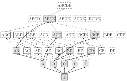
⊥ as its minimum element, thus having a directed acyclic graph (DAG) structure. Given this DAG, one enumeration strategy is to explore the set of candidate patterns following an enumeration tree, spanning the closed patterns (see Figure 2.5, shaded boxes).

⊥

A B C D E

AB AC AD AE BC BD BE CD CE DE

ABC ABD ABE ACD ACE ADE BCD BCE BDE CDE

ABCD ABCE ABDE ACDE BCDE

ABCDE

Figure 2.5: A DAG representation of a set F of patterns defined over a ground set E = {A,B,C,D,E}. In the boxes, the label ACD stands for {A,C,D}. Dashed boxes are candidate patterns, solid boxes are meaningful patterns and shaded boxes are closed pattern. Each dashed edge connects a pattern and its augmentation. The enumeration tree over the set C of closed patterns, is presented in solid edges.