[PENDING] Analytic Properties of Diffraction Gratings Daniel Maystre

(1)

HAL Id: hal-00770372

https://hal.archives-ouvertes.fr/hal-00770372

Submitted on 5 Jan 2013

HAL is a multi-disciplinary open access archive for the deposit and dissemination of sci- entific research documents, whether they are pub- lished or not. The documents may come from teaching and research institutions in France or abroad, or from public or private research centers.

L’archive ouverte pluridisciplinaire HAL, est destinée au dépôt et à la diffusion de documents scientifiques de niveau recherche, publiés ou non, émanant des établissements d’enseignement et de recherche français ou étrangers, des laboratoires publics ou privés.

Daniel Maystre

To cite this version:

Daniel Maystre. Analytic Properties of Diffraction Gratings. E. Popov. Gratings: Theory and Numeric Applications, AMU (PUP), pp.2.1-2.23, 2012, 978-2-8539-9860-4. �hal-00770372�

(2)

GratinGs:

theory and numeric applications

Tryfon Antonakakis Fadi Baïda

Abderrahmane Belkhir Kirill Cherednichenko Shane Cooper

Richard Craster Guillaume Demesy John DeSanto

Gérard Granet

Evgeny Popov, Editor

Boris Gralak

Sébastien Guenneau Daniel Maystre

André Nicolet Brian Stout Gérard Tayeb Fréderic Zolla Benjamin Vial

Institut Fresnel, Université d’Aix-Marseille, Marseille, France Femto, Université de Franche-Compté, Besançon, France LASMEA, Université Blaise Pascal, Clermont-Ferrand, France Colorado School of Mines, Golden, USA

CERN, Geneva, Switzerland Imperial College London, UK Cardiff University, Cardiff, UK

Mouloud Mammeri Univesity, Tizi-Ouzou, Algeria ISBN: 2-85399-860-4

www.fresnel.fr/numerical-grating-book

(3)

ISBN: 2-85399-860-4 First Edition, 2012

World Wide Web:

www.fresnel.fr/numerical-grating-book

Institut Fresnel, Université d’Aix-Marseille, CNRS Faculté Saint Jérôme,

13397 Marseille Cedex 20, France

Gratings: Theory and Numeric Applications, Evgeny Popov, editor (Institut Fresnel, CNRS, AMU, 2012)

(4)

Chapter 2:

Analytic Properties of Diffraction Gratings

Daniel Maystre

(5)

2.1 Introduction . . . . 2.¹ 2.2 From the laws of Electromagnetics to the boundary-value problems . . . . 2.1 2.2.1 Presentation of the grating problem . . . . 2.1 2.2.2 Maxwell’s equations . . . . 2.3 2.2.3 Boundary conditions on the grating profile . . . . 2.4 2.2.4 Separating the general boundary-value problem into two separated scalar

problems . . . . 2.4 2.2.5 The special case of the perfectly-conducting grating . . . . 2.7 2.3 Pseudo-periodicity of the field and Rayleigh expansion . . . . 2.8 2.4 Grating formulae . . . 2.10 2.5 Analytic properties of gratings . . . 2.11 2.5.1 Balance relations . . . 2.11 2.5.2 Compatibility between Rayleigh coefficients . . . 2.14 2.5.3 Energy balance . . . 2.15 2.5.4 Reciprocity . . . 2.16 2.5.5 Uniqueness of the solution of the grating problem . . . 2.18 2.5.6 Analytic properties of crossed gratings . . . 2.19 2.6 Conclusion . . . 2.21 References . . . .�.� .� .��. �.� .� . �. �.� .� .� .� .� .� . �.� .� .� .� .� .� .� .� .� 2.23�

(6)

Analytic Properties of Diffraction Gratings

Daniel Maystre

Institut Fresnel

Campus Universitaire de Saint Jérôme 13397 Marseille Cedex 20, France

daniel.maystre@fresnel.fr

2.1 Introduction

Since the 80’s, specialists of gratings can rely on very powerful grating softwares [1-6]. These softwares are able to compute grating efficiencies for almost any kind of grating in any domain of wavelength, even though the progress of grating technologies needs endless extensions of grating theories to new kinds of structures. These softwares are based on elementary laws of Electromagnetics. Using mathematics, these laws lead to boundary value problems which can be solved on computers using adequate algorithms.

However, a grating user should not ignore some general properties of gratings which can derived directly from the boundary value problem without any use of computer. These analytic properties are valuable at least for two reasons. First, they strongly contribute to a better understanding of an instrument which puzzled and fascinated many specialists of Optics since the beginning of the 20th century. Secondly, they allow a theoretician to check the validity of a new theory or its numerical implementation, although one must be very cautious: a theory can fail while its results satisfy some analytic rules. Specially, this surprising remark apply to properties like energy balance or reciprocity theorem.

The first part of this chapter is devoted to the use of the elementary laws of Electromag- netics for stating the boundary value problems of gratings in various cases of materials and polarizations. Then, we deduce from the boundary value problems the most important analytic properties of gratings.

2.2 From the laws of Electromagnetics to the boundary-value problems 2.2.1 Presentation of the grating problem

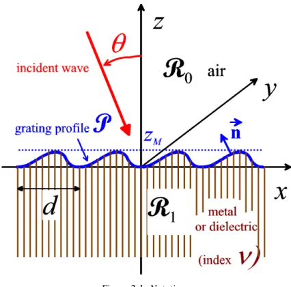
Figure 2.1 represents a diffraction grating. Its periodic profile P of periodd along thex axis separates air (region R0) from a grating material (regionR1) which is generally a metal or a dielectric. Theyaxis is the axis of invariance of the structure and thezaxis is perpendicular to the average profile plane. We denote byz_Mthe ordinate of the top ofP, its bottom being located

(7)

Figure 2.1: Notations.

on the xy plane by hypothesis. We suppose that the incident light can be described by a sum of monochromatic radiations of different frequencies. Each of these can in turn be described in a time-harmonic regime, which allows us to use the complex notation (with an exp(−iωt) time-dependence). In this chapter, we assume that the wave-vector of each monochromatic radiation lies in the cross-section of the grating (xz plane). In the following, we deal with a single monochromatic radiation.

The electromagnetic properties of the grating material (assumed to be non-magnetic) are represented by its complex refractive index ν which depends on the wavelength λ =2πc/ω in vacuum (c=1/√

ε₀µ₀being the speed of light, withε₀ andµ₀ the permittivity and the per- meability of vacuum). This complex index respectively includes the conductivity (for metals) and/or the losses (for lossy dielectrics). It becomes a real number for lossless dielectrics.

In the air region, the grating is illuminated by an incident plane wave. The incident electric field−→

Eⁱis given by :

−

→ Eⁱ=−→

P exp ik₀xsin(θ)−ik₀zcos(θ)

, (2.1)

withθ being the angle of incidence, from thez axis to the incident direction, measured in the counterclockwise sense, andk₀being the wavenumber in the air (k₀=2π/λ, we take an index equal to unity for air). The wave-vector of the incident wave is given by:

−

→ kⁱ₀=





k₀sin(θ) 0

−k₀cos(θ)



. (2.2)

The physical problem is to find the total electric and magnetic fields−→

E and−→

H at any point of space.

(8)

2.2.2 Maxwell’s equations

First, let us notice that the physical problem remains unchanged after translations of the grating or of the incident wave along theyaxis since they do not depend ony. Therefore, if−→

E(x,y,z) and−→

H(x,y,z)are the total fields for a given grating and a given incident wave,−→

E(x,y+y₀,z) and −→

H(x,y+y₀,z) will be solutions too, regardless of the value of y₀. Assuming, from the physical intuition, that the solution of the grating problem is unique, we deduce that−→

E and−→ H are independent ofy.

In order to state the mathematical problem, we use the harmonic Maxwell equations in R0:

∇×−→

E =iω µ₀−→

H, (2.3)

∇×−→

H =−iω ε−→

E, (2.4)

with:

ε=

ε₀ in R0,

ε₁=ε₀ν² in R1. (2.5)

In the following, equations (2.3) and (2.4) will be called first and second Maxwell equations respectively. We note that Maxwell’s equations∇.−→

E =0 and∇.−→

H =0 are the straightforward consequences of the first and second Maxwell equations (it suffices to take the divergence of both members).

We introduce the diffracted fields−→

E^dand−→

H^d defined by:

−→ E^d =

( −→ E −−→

Eⁱ in R0,

−

→E in R1, (2.6)

−→ H^d=

( −→ H−−→

Hⁱ in R0,

−

→H in R1. (2.7)

The interest of the notion of diffracted field is that it satisfies the so-calledradiation condition (or Sommerfeld condition, or outgoing wave condition), in contrast with the total field which does not satisfy this condition in R0 since it includes the incident field. This means that the diffracted fields must remain bounded and propagate upwards inR0 whenz→+∞. The same property must be satisfied in R1, but that time the diffracted fields must remain bounded and propagate downwards in R1 whenz→ −∞. Since the incident fields satisfy Maxwell’s equations inR0, the diffracted fields satisfy these equations as well. Introducing the components of the diffracted fields on the three axes, Maxwell’s equations yield:

∂E_y^d/∂z=−iω µ₀H_x^d, (2.8a)

∂E_y^d/∂x=iω µ₀H_z^d, (2.8b)

∂E_z^d/∂x−∂E_x^d/∂z=−iω µ₀H_y^d, (2.8c)

∂H_y^d/∂z=iω εE_x^d, (2.9a)

∂H_y^d/∂x=−iω εE_z^d, (2.9b)

∂H_z^d/∂x−∂H_x^d/∂z=iω εE_y^d. (2.9c)

(9)

2.2.3 Boundary conditions on the grating profile

On the grating profile, the tangential component of the electric and magnetic fields must be continuous¹. Thus the boundary condition is given by:

(−−−→

[E^d]₀+−−→

[Eⁱ]₀)× −→n =−−−→

[E^d]₁× −→n, (2.10)

(

−−−→

[H^d]₀+−−→

[Hⁱ]₀)× −→n =

−−−→

[H^d]₁× −→n, (2.11)

with −→n being the unit normal to P, oriented toward region R0 (figure 2.1) and the symbol [−→

F]_p denoting the limit of−→

F when a point of regionRptends to the grating profile (with p∈ (0,1)). As for Maxwell’s equations, we note that the other boundary conditions on the normal components of the fields are consequences of equations (2.10) and (2.11). It is worth noting that the linkage between these two boundary conditions is a typical example of an elementary property which is difficult to establish, at least for those who are not acquainted with the theory of distributions. Projecting equations (2.10) and (2.11) on the three axes yields:

[E_y^d]₀−[E_y^d]₁=−[E_yⁱ]₀, (2.12a) n_x[E_z^d]₀−n_z[E_x^d]₀−n_x[E_z^d]₁+n_z[E_x^d]₁=−n_x[E_zⁱ]₀+n_z[E_xⁱ]₀, (2.12b)

[H_y^d]₀−[H_y^d]₁=−[H_yⁱ]₀, (2.13a) n_x[H_z^d]₀−n_z[H_x^d]₀−n_x[H_z^d]₁+n_z[H_x^d]₁=−n_x[H_zⁱ]₀+n_z[H_xⁱ]₀. (2.13b) 2.2.4 Separating the general boundary-value problem into two separated scalar problems The first conclusion to draw from equations (2.8), (2.9), (2.12) and (2.13) is that they can be separated into two independent sets. The first one, called TE case, includes equations (2.8a), (2.8b), (2.9c), (2.12a) and (2.13b). It only contains the transverse component (viz. the y-component)E_y^d of the electric field and thexzcomponents (orthogonal to theyaxis)H_x^d and H_z^dof the magnetic field. It must be remembered that the incident field−→

Eⁱ is given by equation (2.1) and thus is not an unknown field. The same remark applies to the complementary set (TM case), but with the transverse component of the magnetic field and the xzcomponents of the electric field. As a consequence, the general problem of diffraction by a grating can be decomposed into two elementary mathematical problems.

2.2.4.1 The TE case problem

In the first one, the xz components of the magnetic field can be expressed as functions of the transverse component of the electric field using equations (2.8a) and (2.8b). Inserting their expression in equation( 2.9c) shows thatE_y^d satisfies a Helmholtz equation:

∇²E_y^d+k²E_y^d=0, (2.14)

1The continuity of the tangential component of the magnetic field is valid for materials having bounded values of permittivity. When the permittivity of the grating material is infinite, as in the model of perfectly conducting material, this condition does not hold.

(10)

with:

k=

k₀ in R0,

k₁=k₀ν in R1. (2.15)

The associated boundary condition on the diffracted electric field can be deduced from equations (2.12a) and (2.1):

h E_y^d

i

0−h E_y^d

i

1=−P_yexp ik₀xsin(θ)−ik₀zcos(θ)

, with(x,z)∈P, (2.16) while the associated boundary condition on its normal derivative can be deduced from equations (2.13b), (2.8a) and (2.8b):

"

dE_y^d dn

#

0

−

"

dE_y^d dn

#

1

=−

"

dE_yⁱ dn

#

0

,

=−iP_y−→n.−→

k₀ⁱ exp ik₀xsin(θ)−ik₀zcos(θ)

, with(x,z)∈P,

(2.17)

with dF

dn denoting the normal derivative −→

n.∇F. It can be noticed that equation (2.17) entails

the continuity of the normal derivative of the transverse component of the total electric field.

Equations ( 2.14), (2.16) and (2.17) are not sufficient to define the boundary-value problem for TE case. A fourth condition must be added: the radiation condition:

E_y^dmust satisfy a radiation condition forz→ ±∞. (2.18) The boundary value problem allows us to deduce a fundamental property of gratings. Let us suppose that the incident field is TE polarized, i.e. that the electric incident field is parallel to theyaxis (P_x=P_z=0). In these conditions, the equations associated with the TM case are homogeneous: they do not contain the incident field since the right-hand member of equation (2.12b) vanishes. If we believe that the solution of the grating problem is unique, it must be concluded that the xzcomponent of the diffracted and total electric field vanish. On the other hand, the magnetic field is parallel to thexzplane. In other words,in the TE case, the grating problem becomes scalar: we must determine the y-component of the diffracted electric field. Thexzcomponents of the magnetic field deduce they-component of the diffracted electric field using equations (2.8a) and (2.8b).

2.2.4.2 The TM case problem

Now, let us deal with the TM case. As for the TE case, it can be shown that they-component of the magnetic field satisfies a Helmholtz equation by using equations (2.8c), (2.9a) and (2.9b):

∇²H_y^d+k²H_y^d=0. (2.19)

The boundary conditions need the calculation of the incident magnetic field. From equation (2.1) and Maxwell equation (2.3), it turns out that:

−

→ Hⁱ=−→

Qexp ik₀xsin(θ)−ik₀zcos(θ)

, (2.20)

(11)

with:

−

→Q = 1 ω µ₀

−

→ k₀ⁱ.−→

Pexp ik₀xsin(θ)−ik₀zcos(θ)

. (2.21)

The associated boundary condition on the diffracted magnetic field can be deduced from equations (2.13a) and (2.20):

[H_y^d]₀−[H_y^d]₁=−Q_yexp ik₀xsin(θ)−ik₀zcos(θ)

, with(x,z)∈P, (2.22) while the boundary condition on its normal derivative is obtained by inserting the expressions of the xz components of the electric field (equations (2.9a) and (2.9b)) in equation (2.12b).

Remarking that the incident field satisfies the same equations, we obtain finally:

1 ε₀

"

dH_y^d dn

#

0

− 1 ε₁

"

dH_y^d dn

#

1

=−1 ε₀

"

dH_yⁱ dn

#

0

,

=−iQ_y ε₀

−

→n.−→

, with(x,z)∈P.

(2.23)

It can be noticed that equation (2.23) has a simple interpretation: the product 1 ε

dHy

dn is continuous across the profile. Finally, the radiation condition yields:

H_y^dmust satisfy a radiation condition forz→ ±∞. (2.24) Equations (2.19), (2.22), (2.23) and radiation conditions forz→ ±∞define the boundary- value problem for TM case. As for TE case, the uniqueness of the solution shows that that when the magnetic incident field is parallel to theyaxis (Qx=Q_z=0), the equations associated with the TE case are homogeneous: they do not contain the incident field. It can be concluded that the xz components of the diffracted and total magnetic fields vanish. On the other hand, the electric field is parallel to the xzplane. In other words,in the TM case, the grating problem becomes scalar: we must determine the y-component of the diffracted magnetic field. The xzcomponents of the electric field deduce from they-component of the diffracted magnetic field using equations (2.9a) and (2.9b).

2.2.4.3 TE and TM cases: a unified presentation of the boundary-value problem

In order to deal with both cases simultaneously, we denote byF^d the field defined by:

F^d=

E_y^d for TE case,

H_y^d for TM case. (2.25)

In the same way, by assuming that the incident field has a unit amplitude (P_y=1 for TE case and Q_y=1 for TM case), the incident field in both cases is given by:

Fⁱ=exp ik₀xsin(θ)−ik₀zcos(θ)

, (2.26)

the total fieldF being given by:

F=

F^d+Fⁱ in R0,

F^d in R1. (2.27)

(12)

Using equations (2.14), (2.16), (2.17), (2.18), (2.19), (2.22), (2.23) and (2.24), it is possible to gather both cases in a unique set of equations:

∇²F^d+k²F^d=0, h

F^d i

0−h F^d

i

1=−exp ik₀xsin(θ)−ik₀zcos(θ)

with(x,z)∈P, 1

τ₀ dF^d

dn

0

− 1 τ₁

dF^d dn

1

,

=− i τ₀

−

→n.−→

kⁱ₀exp ik₀xsin(θ)−ik₀zcos(θ)

, with(x,z)∈P, F^d must satisfy a radiation condition fory→ ±∞,

(2.28) (2.29)

(2.30)

(2.31) with:

τ_i=

1 for TE case,

ε_i for TM case,i∈(0,1). (2.32)

In the following, this boundary-value problem will be called normalized grating problem. It is worth noting that equations (2.29) and( 2.30) take a simpler form by introducing the total field F:

[F]₀= [F]₁, (2.33)

1 τ0

dF dn

0

= 1 τ1

dF dn

1

. (2.34)

2.2.5 The special case of the perfectly-conducting grating

The first grating theories were devoted to perfectly conducting gratings. This case is very important since it is realistic for metallic gratings in the microwave domain and far infrared regions.

In the visible and infrared regions, it can provide qualitative results. However, in these regions, one must be very cautious. The existence of surface plasmons propagating at the vicinity of the grating surface generates strong resonance phenomena for TM case. Due to these phenomena, the properties of real metallic gratings and those of perfectly-conducting gratings may completely differ[2].Moreover, the perfect conductivity model allows one to simplify the grating theory, since the associated boundary-value problems are much simpler.

Basically, the equations associated to the perfect conductivity model are the same as for real metallic or dielectric gratings, except equations (2.4) and (2.11). Let us give a brief expla- nation to this property. In Maxwell equation (2.4), the right-hand member includes the volume current density −→

j in the metal since this term is proportional to the electric field (−→

j =σ−→ E, σ being the conductivity of the metal). When the conductivity tends to infinity, the volume current density and the total fields concentrate more and more on the grating surface since the skin depth tends to zero. As a consequence, at the limit when the conductivity tends to infinity, the fields are null in R1 while the volume current density −→

j becomes a surface current density−→

j_P. This surface current density cannot be included in the right-hand member of equation (2.4) since it is a singular distribution (for the specialist of Schwartz distributions [7], it writes

−→

j_Pδ_P). Finally, equation (2.4) becomes:

∇×−→

H =−iωε˜−→ E +−→

j_P, (2.35)

(13)

with ˜ε being the permittivity of the material. Furthermore, taking into account that the total fields vanish insideR1, the boundary condition (equation (2.11)) becomes:

−

→n ×(

−−−→

[H^d]₀+

−−→

[Hⁱ]₀) =−→

j_P. (2.36)

This equation reduces to a relation between the surface current density on P and the limit of the magnetic field aboveP. It does not constitute any more an element of the boundary-value problem.

In conclusion, for perfectly conducting gratings, the fields inside R1 vanish and, using equations (2.3), (2.4), (2.10), (2.6) and (2.7), the basic vector equations for the field inR0 can be written:

∇×−→

E^d=iω µ₀

−→

H^d, (2.37)

∇×−→

H^d=−iω ε₀−→

E^d, (2.38)

(

−−−→

[E^d]₀+−−→

[Eⁱ]₀)× −→n =0. (2.39)

Following the same lines as in subsections 2.2.4.1 and 2.2.4.2, the boundary value problems for perfectly conducting gratings are given by:

For TE case:

∇²E_y^d+k²₀E_y^d=0, h

E_y^d i

0=−P_yexp ik₀xsin(θ)−ik₀zcos(θ)

, with(x,z)∈P, E_y^dmust satisfy a radiation condition forz→+∞.

(2.40) (2.41) (2.42) For TM case:

∇²H_y^d+k²₀H_y^d=0,

"

dH_y^d dn

#

0

=−iQ_y−→n.

−

→

, with(x,z)∈P,

H_y^dmust satisfy a radiation condition forz→+∞.

(2.43) (2.44) (2.45) 2.3 Pseudo-periodicity of the field and Rayleigh expansion

This section establishes the most famous property of diffraction gratings: the dispersion of light, which is a consequence of the well known grating formula. In general, this formula is demonstrated using heuristic considerations of physical optics. Here, we propose a rigorous demonstration based on the boundary-value problem stated in subsection 2.2.4.3. First, let us show that the fieldF^dis pseudo-periodic, i.e. that:

F^d(x+d,z) =F^d(x,z)exp ik₀dsin(θ)

. (2.46)

With this aim, we consider the functionG(x,z)defined by:

G(x,z) =F^d(x+d,z)exp −ik₀dsin(θ)

. (2.47)

(14)

The pseudo-periodicity ofF^dis proved if we show thatF^d(x,z) =G(x,z). Owing to the uniqueness of the solution of the boundary-value problem defined by equations (2.28), (2.29), (2.30) and (2.31), this equation is satisfied ifGobeys the same equations. Obviously,Gsatisfies these equations sincedis the grating period. ThusF^d is pseudo-periodic, with coefficient of pseudo- periodicity k₀sin(θ), as well asFⁱ and F. Notice that in normal incidence (θ =0), pseudo- periodicity becomes ordinary periodicity, which in that case is a straightforward property since both grating and incident wave are periodic.

Using the pseudo-periodicity, let us show that the field above and below the grating is a sum of plane waves. With this aim, we notice from equation (2.28) thatF^d(x,z)exp −ik₀xsin(θ) has a periodd and thus can be expanded in a Fourier series:

F^d(x,z)exp −ik₀xsin(θ)

=

+∞

n=−∞

∑

F_n^d(z)exp(2iπnx/d). (2.48) Multiplying both members of equation (2.48) by exp ik₀xsin(θ)

yields : F^d(x,z) =

+∞

n=−∞

∑

F_n^d(z)exp(iα_nx), (2.49)

with:

α_n=k₀sin(θ) +2πn/d. (2.50)

Introducing this expression ofF^d(x,z)in Helmholtz equation (2.28), we find :

+∞

n=−∞

∑

d²F_n^d(z)/dz²+ (k²−α_n²)F_n^d(z)

exp(iα_nx) =0, (2.51) and multiplying both members by exp −ik₀xsin(θ)

,

+∞

n=−∞

∑

d²F_n^d(z)/dz²+ (k²−α_n²)F_n^d(z)

exp(2iπnx/d) =0. (2.52) It seems, at the first glance, that the left-hand member of equation (2.52) is a Fourier series, and thus that the coefficients of this Fourier series vanish. This is not correct. Indeed, we have to bear in mind thatk, defined in equation (2.15) is not a constant. As a consequence, if 0<y<z_M, a region called intermediate region in the following,k²depends onxand the left-hand member of equation (2.52) is not a Fourier series. However, above and below this intermediate region, k²is constant and we can write that the Fourier coefficients vanish:

∀n, d²F_n^d(z)/dz²+γ_0,n² F_n^d(z) =0 ify>z_M, (2.53a)

∀n, d²F_n^d(z)/dz²+γ_1,n² F_n^d(z) =0 ify<0, (2.53b) with:

γ_i,n= q

(k²_i −α_n²) i∈(0,1). (2.54)

We deduce that:

F_n^d(z) =

I_0,nexp(−iγ_0,nz) +D_0,nexp(+iγ_0,nz) ify>z_M,

D_1,nexp(−iγ_1,nz) +I_1,nexp(+iγ_1,nz) ify<0, (2.55)

(15)

and therefore, using equation (2.49),

F^d(x,z) =











∑^+∞_n=−∞ I_0,nexp(iα_nx−iγ_0,nz)+

+D_0,nexp(iα_nx+iγ_0,nz)

ifz>z_M,

∑^+∞_n=−∞ D_1,nexp(iα_nx−iγ_1,nz)+

+I_1,nexp(iα_nx+iγ_1,nz)

ifz<0.

(2.56)

Let us remark that equation (2.54) does not assign to γi,n a unique value. However, equation (2.56) shows that its determination can be chosen arbitrarily since a sign change does not modify the value of the field, provided that I_0,n and D_0,n are permuted. The determination of these constants will be given by:

Re(γ_i,n) +Im(γ_i,n)>0, i∈(0,1), (2.57) with Re(q)and Im(q)denoting the real and imaginary parts ofq.

Equation (2.56) shows that the field above and below the intermediate region can be represented by plane wave expansions. The propagation constants of the plane waves along the x andzaxes are respectively equal toαnand±γ_i,n. In the physical problem, some of these plane waves must be rejected since they do not obey the radiation condition. This condition entails that I_0,n=I_1,n=0 since, according to equation (2.57), the associated plane waves propagate towards the grating profile. Finally, equations (2.56), (2.27) and the radiation condition allow us to express the total field by adding the incident field:

F(x,z) =







exp(iα₀x−iγ_0,0z)+

+∑^+∞_n=−∞D_0,nexp(iα_nx+iγ_0,nz) ifz>z_M,

∑^+∞_n=−∞D_1,nexp(iα_nx−iγ_1,nz) ifz<0,

(2.58) the sums being the expression of the scattered field in both regions. The unknown complex coefficientsD_0,nandD_1,nare the amplitudes of the reflected and transmitted waves respectively.

The conclusion of this subsection is that above and below the intermediate region, the field reflected and transmitted by the grating takes the form of sums of plane waves (Rayleigh expansion [8]), each of them being characterized by its ordern.

2.4 Grating formulae

According to equation (2.54), almost all the diffracted plane waves (an infinite number) are evanescent: they propagate along the x axis at the vicinity of the grating profile since they decrease exponentially when |z| →+∞. For z→+∞, they correspond to the orders n such that α_n² ≥k²₀, thus rendering γ_0,n =i

q

(α_n²−k²₀) a purely imaginary number. Only a finite number of them, calledz-propagative orders, propagate towardsz= +∞, withα_n²≤k²₀ , thus γ_0,n=

q

(k²₀−α_n²) being real. Let us notice that among these orders, the 0^th order is always included, sinceγ0,n=k₀cos(θ). It propagates in the direction specularly reflected by the mean plane of the profile, whatever the wavelength may be. In contrast, the otherz-propagative orders are dispersive. Indeed, their propagation constants along thex andz axes are equal toα_n and γ0,n, in such a way that the diffraction angleθ0,n of one of these waves, measured clockwise from the z axis, can be deduced fromα_n=k₀sin(θ_0,n). Using the expression ofα_n given by equation (2.50), the angle of diffraction is given by :

sin(θ_0,n) =sin(θ) +n2π

k₀d =sin(θ) +nλ

d. (2.59)

(16)

This is the famous grating formula, often deduced from heuristic arguments of physical optics.

For the field below the grooves, the wavenumberk₀ is replaced byk₁=k₀ν. If the grating material is a lossless dielectric, the directions of propagation of the transmitted field obey a grating formula as well. This formula is similar to equation (2.59) but the angles of transmission θ1,n can be deduced from αn=k₀νsin(θ_1,n), which yields, using a counterclockwise convention:

νsin(θ_0,n) =sin(θ) +n2π

k₀d =sin(θ) +nλ

d. (2.60)

The 0^th order is always included in thez-propagative orders². It propagates in the direction of transmission by an air/dielectric plane interface, whatever the wavelength may be. In contrast, the otherz-propagative orders are dispersive. When the grating material is metallic, the transmitted plane waves are absorbed by the metal and thez-propagating orders below the grooves no longer exist.

In conclusion of this section, the reflected and transmitted fields include, outside the grooves, a finite number of plane waves propagating to infinity with scattering angles given by the grating formulae. All the orders are dispersive, except the0^th orders. The reflected 0^thorder takes the specular direction while for a lossless material, the transmitted 0^thorder takes the direction transmitted by an air/dielectric plane interface. Consequently, a polychromatic incident plane wave generates in a given order n different from 0 a sum of plane waves scattered in different directions, i.e. a spectrum. The measurement of the intensity along this spectrum allows one to determine the spectral power of the incident wave. This dispersion phenomenon is the most important property of diffraction gratings. It explains why this optical component has been one of the most valuable tools in the history of Science.

2.5 Analytic properties of gratings 2.5.1 Balance relations

The mathematical balance relations established in this subsection will allow us to demonstrate very important general properties of gratings. These balance relations state mathematical links between characteristics of the field in two regions separated by large distances, without consid- ering the fields in between. They can give a relation between the fields atz= +∞and the fields on the grating profile, or the fields at z=−∞and the fields on the grating profile, or the fields atz= +∞andz=−∞.

2.5.1.1 Lemma 1

We consider two pseudoperiodic functionsuandvof the two variables xandz, defined inR0, which belong to the classG₀of functions having the following properties:

• They are pseudo-periodic, with the same coefficient of pseudo-periodicity α, in other words,u(x,z)exp(−iαx)andv(x,z)exp(−iαx)are periodic,

2This property does not hold if the upper medium is not air but has an index ˜ν greater than the indexνof the lower medium, provided that the incidence is chosen in such a way that the incident wave is totally reflected by a plane interface (Total Internal Reflection). In that case, sin(θ)is replaced by ˜νsin(θ)in equation (2.60), in such a way that the zeroth order is evanescent if ˜νsin(θ)>ν.

(17)

• They are solutions of a Helmholtz equation:

∇²u+k²₀u=0, (2.61a)

∇²v+k²₀v=0, (2.61b)

withk₀being real.

• They are bounded forz→∞,

• They are square integrable inxand locally square integrable inz,

• Their values onP are square integrable, as well as their normal derivatives.

We introduce the sesquilinear functional defined by:

F0= Z

P

udv

dn−vdu dn

ds. (2.62)

The symbol ^R_P denotes a curvilinear integral on one period of the profile P of the grating, with dsbeing the differential of the curvilinear abscissa onP. Obviously, the value in region R0 of the fields F(x,z), solutions of the four boundary-value problems defined in subsection 2.2.4, belong to G₀, as well as the incident field Fⁱ. It is to be noticed that we do not impose a boundary condition on P or a radiation condition at infinity, but we still impose that these functions must remain bounded at infinity.

Following the same lines as in section 2.3, it can be shown that above the top of the grooves, u and v can be represented by plane wave expansions, similar to that of equation (2.56): ifz>z_M,

u(x,z) =

+∞

n=−∞

∑

[I_0,nexp(iα_nx−iγ_0,nz) +D_0,nexp(iα_nx+iγ_0,nz)], (2.63a)

v(x,z) =

+∞

n=−∞

∑

[I_0,n⁰ exp(iα_nx−iγ_0,nz) +D⁰_0,nexp(iα_nx+iγ_0,nz)]. (2.63b) Let us notice that some terms must be eliminated in the Rayleigh expansions. Indeed, the field must remain bounded at infinity. It is not the case for the incident terms of coefficientsI_0,nand I_0,n⁰ unless the corresponding plane waves arez-propagating waves. Thus we define the setU₀ of orders corresponding toz-propagating waves and equations (2.63) become:

u(x,z) =

∑

n∈U0

I_0,nexp(iα_nx−iγ_0,nz) +

+∞

n=−∞

∑

D_0,nexp(iα_nx+iγ_0,nz), (2.64a)

v(x,z) =

∑

n∈U₀

I_0,n⁰ exp(iα_nx−iγ_0,nz) +

+∞

n=−∞

∑

D⁰_0,nexp(iα_nx+iγ_0,nz), (2.64b)

v(x,z) =

∑

n∈U0

I_0,n⁰ exp(−iα_nx+iγ_0,nz)+

+

+∞

n=−∞

∑

D⁰_0,nexp(−iα_nx−iγ_0,nz).

(2.64c)

(18)

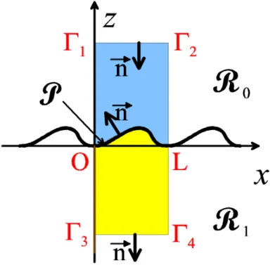
Figure 2.2: Balance relations.

Now, we show that F0 can be expressed as a function of the Rayleigh coefficients I_0,n, D_0,n,I_0,n⁰ andD⁰_0,n. With this aim, we multiply equation (2.61a) byv, the conjugate of equation (2.61b) byuand we substract the first from the second, which yields:

u∇²v−v∇²u=0 in R0. (2.65)

Integrating equation (2.65) in the blue area of figure 2.2 and applying the second Green identity yields:

Z

Ω0

udv

dn−vdu dn

dl=0, (2.66)

with Ω₀ being the boundary of the blue area of figure 2.2 and dl denoting the differential of the curvilinear abscissa onΩ₀. According to equations (2.64a) and (2.64c), udv

dx and vdu dx are periodic. Since the orientations of the normal on verticals OΓ₁and LΓ₂ are opposite, the contributions of the integrals on these segments cancel each other. Furthermore, the normal to OΓ₁ and LΓ₂is parallel to thezaxis and oriented downwords, then equation (2.66) becomes:

Z

P

udv

dn−vdu dn

ds=

Z

Γ1Γ2

udv

dz−vdu dz

dx. (2.67)

Introducing in the right-hand member of equation (2.66) the expressions of u and v given by equations (2.64a) and (2.64c), separating the termsn∈U₀ from the other ones and taking into account that^R_x=0^d expin^2π_d x=δ_n,0, withδ_n,0being the Kronecker symbol, one can obtain, after some cumbersome but not difficult calculations that:

Z

P

udv

dn−vdu dn

ds=

∑

n∈U0

γ_0,n(I_0,nI_0,n⁰ −D_0,nD⁰_0,n). (2.68)

(19)

2.5.1.2 Lemma 2

In this section, it is supposed that the grating material is lossless, in such a way that plane waves can propagate inR1. Lemma 2 is similar as lemma 1, but for regionR1. We denote byU₁ the set of orders corresponding toz-propagating waves inR1. The expressions ofuandvbelow the x axis are given by:

u(x,z) =

∑

n∈U₁

D_1,nexp(iα_nx−iγ_1,nz) +

+∞

n=−∞

∑

I_1,nexp(iα_nx+iγ_1,nz), (2.69a)

v(x,z) =

∑

n∈U₁

D⁰_1,nexp(iα_nx−iγ_1,nz) +

+∞

n=−∞

∑

I_1,n⁰ exp(iα_nx+iγ_1,nz), (2.69b)

v(x,z) =

∑

n∈U1

D⁰_1,nexp(−iα_nx+iγ_1,nz)+

+

+∞

n=−∞

∑

I_1,n⁰ exp(−iα_nx−iγ_1,nz).

(2.69c)

Following the same lines as in section 2.5.1.1 but for the yellow area of figure 2.2 and noting that the normal is now oriented towards the exterior of the domain, it can be deduced that:

Z

P

udv

dn−vdu dn

ds=−

∑

n∈U1

γ_1,n(I_1,nI_1,n⁰ −D_1,nD⁰_1,n). (2.70)

2.5.2 Compatibility between Rayleigh coefficients

In order to state a relation between the Rayleigh coefficients above and below the grating profile, we assume that the functionsuandvsatisfy the boundary conditions imposed on the total fields by equations (2.33) and (2.34). On the other hand, we do not impose radiation conditions at infinity, but the functions must remain bounded. In other words,uandv can be considered as solutions of the most general grating problem, in which the incident wave is not restricted to a single plane wave, but to the sum of all the plane waves generating diffracted waves in the same directions, with arbitrary amplitudes. It is straightforward to show from equations (2.33) and (2.34) that the left-hand members of equations (2.68) and (2.70) are proportional, then to deduce a relation including the coefficients of the Rayleigh expansions of the field only:

1 τ₀

∑

n∈U0

γ0,n(I_0,nI_0,n⁰ −D_0,nD⁰_0,n)+

1 τ1

∑

n∈U1

γ_1,n(I_1,nI_1,n⁰ −D_1,nD⁰_1,n) =0.

(2.71)

This equation states the most general relation of compatibility between two solutions of the general diffraction grating problem associated to different sets of incident waves. When the grating material is perfectly conducting, it is easy to show that the compatibility equation holds, provided that the sumn∈U₁is cancelled in equation (2.71).

(20)

Phenomenological theories of gratings make a wide use of the notion of scattering matrix (or S-matrix). The scattering matrix states the linear relation between the amplitudes of the diffracted and incident waves. We define the column matrix containing the amplitudes of the incident waves. More precisely, we define the normalized amplitudes of the incident and scattered waves by ˜I_0,n=√

γ0,nI_0,n, ˜D_0,n=√

γ0,nD_0,n, ˜I_1,n= rτ₀

τ₁γ1,nI_1,n, ˜D_1,n= rτ₀

τ₁γ1,nD_1,n, n∈(0,1), and by definition, the scattering matrix is a square matrix defined by:

D=SI, (2.72)

withIbeing a column vector containing successively all the incident amplitudes ˜I_0,nforn∈U₀ and all the incident amplitudes ˜I_1,nforn∈U₁,Dbeing a column vector containing successively all the diffracted amplitudes ˜D_0,n, and all the incident amplitudes ˜D_1,n for n∈U₁ . Thus, the order of column matrices I andD is the sum|U₀|+|U₁| of the cardinals ofU₀ andU₁ Using these notations, equation (2.71) can be expressed in the very simple form:

<D|D⁰>=<I|I⁰>, (2.73)

the scalar product of two column matrices of orderN being defined by:

<P|Q>=

N

∑

j=1

P_jQ_j. (2.74)

Using equation (2.72) to eliminateDin equation (2.77) yields:

<SI|SI⁰>=<(S^∗S)I|I⁰>=<I|I⁰>, (2.75) withS^∗being the adjoint matrix ofS. Since equation (2.75) must be satisfied for any value ofI andI⁰, we deduce that:

S^∗S=1, (2.76)

with1being the identity matrix. Equation (2.76) shows thatSis unitary.

2.5.3 Energy balance

The energy balance relation is obtain by takingu=vin equation (2.77), which gives:

<D|D>=<I|I>, (2.77)

or equivalently:

kDk=kIk. (2.78)

Let us show why this equation is known as energy balance relation. To this end, it suffices to use the Poynting theorem and to calculate the flux of the Poynting vector−→

E ×−→

H through the rectangleΓ₁Γ₂Γ₄Γ₃of figure 2.2. Since the grating material is lossless, the flux of the Poynting vector through this rectangle (with now the normal oriented toward the exterior, in contrast with figure 2.2) must be null. The contributions of the vertical sides Γ₁Γ₃ and Γ₂Γ₄ cancel each other, thanks to the periodicity of the Poynting vector (−→

H has a coefficient of pseudo- periodicity which is the opposite to that of −→

E). At the top of the rectangle, the calculation of the flux of the Poynting vector can be achieved by using the Rayleigh expansion given by

(21)

equations (2.64). Taking into account that ^R_x=0^d expin^2π_d x=δ_n, elementary calculations show that the contributions to this flux of the different plane waves are decoupled and are proportional to−γ_0,n|I_0,n|²and+γ_0,n|D_0,n|². At the bottom of the rectangle, we use the Rayleigh expansion given by equations (2.69). The contributions of the plane waves are decoupled as well and are proportional to −τ₀

τ₁γ1,n|I_1,n|² and+τ₀

τ₁γ1,n|D_1,n|², with the same coefficient of proportionality as the contributions on the top of the rectangle. Therefore, the energy balance can be written:

n∈U

∑

0

γ_0,n|D_0,n|²+

∑

n∈U1

τ₀ τ1

γ_1,n|D_1,n|²=

=

∑

n∈U₀

γ0,n|I0,n|²+

∑

n∈U₁

τ₀

τ₁γ1,n|I1,n|².

(2.79)

The first and second terms in the left-hand member of equation (2.79) represent the energy diffracted upwards and downwords respectively and the corresponding terms in the right-hand member are the incident energy propagating downwords and upwards respectively.

Coming back to the physical problem where the incident wave is unique and has a unit amplitude (see equation (2.26)), equation (2.79) becomes:

n∈U

∑

0

γ_0,n|D_0,n|²+

∑

n∈U1

τ₀

τ₁γ_1,n|D_1,n|²=γ_0,0, (2.80) the right-hand member representing the incident energy. In that case, the efficiency ρ_i,n, i∈ (0,1)is defined as the ratio of the energy diffracted in a given order over the incident energy.

Using equation (2.79) yields:

ρi,n=





 γ_0,n

γ_0,0|D_0,n|² ifi=0, τ0

τ₁ γ_1,n

γ_0,0|D_1,n|² ifi=1, (2.81)

and the energy balance can be written:

n∈U

∑

0

ρ0,n+

∑

n∈U1

ρ1,n=1. (2.82)

The sum of efficiencies is equal to unity.When the grating is perfectly conducting, it is easy to show that the energy balance still holds, provided that the sumn∈U₁is cancelled in equations (2.79), (2.80) and (2.82). When the grating material is lossy, the sumn∈U₁must be cancelled as well and one can show that equation (2.82) becomes:

n∈U

∑

0

ρ_0,n<1. (2.83)

The sum of reflected efficiencies is smaller than one, a rather intuitive result if we bear in mind that a part of the incident energy is dissipated in the grating material.

2.5.4 Reciprocity

In order to demonstrate the well known reciprocity relation, we consider a functionu, sum of the solution of the normalized grating problem (see equations( 2.28), (2.29), (2.30) and (2.31))

(22)

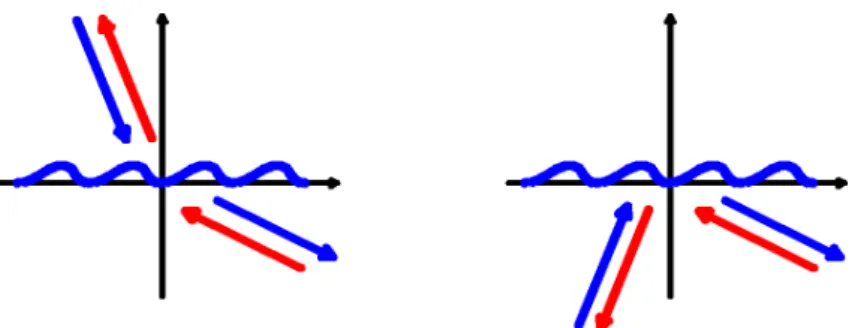
Figure 2.3: The reciprocity theorem: The efficiency in the p^thorder is the same in the two cases symbolized by red and blue arrows.

and of the corresponding incident field (in other words,uis the total field). In order to definev, we consider the p^th order of diffraction (p∈U₀) inR0, with diffraction angleθ0,p.

Then, we consider a second problem, but with angle of incidenceθ⁰⁰=−θ_0,p, as shown³ in figure 2.3. The incident wave in this second case has a direction of propagation which is just the opposite of that of the p^th diffracted order in the first case and straightforward calculations show that the corresponding p^th order inR0 has a direction of propagation which is the opposite of that of the incident wave in the first case, which entailsθ_0,p⁰⁰ =−θ. This geo- metrical property is known in optics as the reversion theorem. The constants of propagation of the p^th diffracted order in this second case are given by α_p⁰⁰ =−α₀ and γ_0,p⁰⁰ =γ0,0 and more generally, the constants of propagation of an arbitraryn^th diffracted order in this second case are given byα_n⁰⁰=−α_p−nandγ_0,⁰⁰_n =γ_0,p−n. Thusv⁰⁰can be written:

v⁰⁰(x,z) =exp(−iα_px−iγ_0,pz) +

+∞

n=−∞

∑

D⁰⁰_0,nexp(−iα_p−nx+iγ_0,p−nz). (2.84)

Functionsuandv⁰⁰do not satisfy the conditions of the equation of compatibility (equation (2.71)) since they have not the same pseudo-periodicity. It is not so foruand the functionv=v⁰⁰ which is given by:

v(x,z) =exp(iα_px+iγ_0,pz) +

+∞

n=−∞

∑

D⁰⁰_0,nexp(iα_p−nx−iγ_0,p−nz). (2.85)

3It must be remembered that the conventions for the measurements of the angles of incidence and diffraction inR0are opposite

(23)

Figure 2.4: Other reciprocity relations: The efficiency is the same in the two cases symbolized by red and blue arrows.

Identifying the incident and diffracted waves in equation (2.85) yields:

I_0,n⁰ =D⁰⁰_0,p−n, (2.86a)

D⁰_0,n=δn−p, (2.86b)

and from equation (2.71), it turns out that:

γ_0,p⁰⁰ D⁰⁰_0,p=γ0,pD_0,p. (2.87) This is the reciprocity theorem: the products of the amplitudes of the plane waves represented in figure 2.3 by their propagation constants along thezaxis is invariant. In order to state the reciprocity theorem in a form which is most widespread, we take the modulus square of both members of equation (2.87):

γ_0,p⁰⁰ ²|D⁰⁰_0,p|²=γ_0,p²|D_0,p|². (2.88) Writing equation (2.88) in the form:

γ_0,p⁰⁰ γ0,p

|D⁰⁰_0,p|²= γ0,p

γ_0,p⁰⁰ |D_0,p|², (2.89)

and bearing in mind thatγ0,p=γ_0,0⁰⁰ andγ_0,p⁰⁰ =γ0,0, and using the definition of the efficiencies given in equation (2.81), equation (2.89) yields:

ρ_0,p⁰⁰ =ρ0,p. (2.90)

The efficiency is invariant.

Figure 2.4 illustrates two other cases where the reciprocity theorem applies. These properties can be demonstrated by following the same lines as in the first part of this section. It is important to notice that the reciprocity theorem illustrated in figure 2.3 holds for lossy materials [9]. More surprisingly, the theorem can be generalized to evanescent waves [10].

2.5.5 Uniqueness of the solution of the grating problem

If two different solutions of the normalized grating problem exist, their differencew(x,z)does not include any incident wave. We will show that such a field vanish. We assume here that the

(24)

grating material is lossless. First, using the compatibility equation (2.71) with u=v=w, it emerges that:

1 τ0

∑

n∈U0

γ_0,n|D_0,n|²+ 1 τ1

∑

n∈U1

γ_1,n|D_1,n|²=0. (2.91) Sinceτ₀, τ₁, γ_0,nandγ_1,nare positive, equation (2.91) implies thatD_0,n=D_1,n=0. This is an important result since it means that ifwexists, it has no effect on the far field: the solution in the far field is unique. However, it could exist a function wlocalized at the vicinity of the grating profile and tending to zero exponentially at infinity. The interested reader can find a complete and not straightforward demonstration of the uniqueness in [1], at least for the TE case.

2.5.6 Analytic properties of crossed gratings

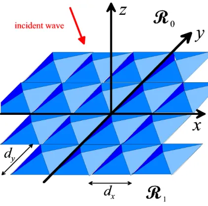
Figure 2.5: A crossed grating with periods d_xand d_zon the x and z axes.

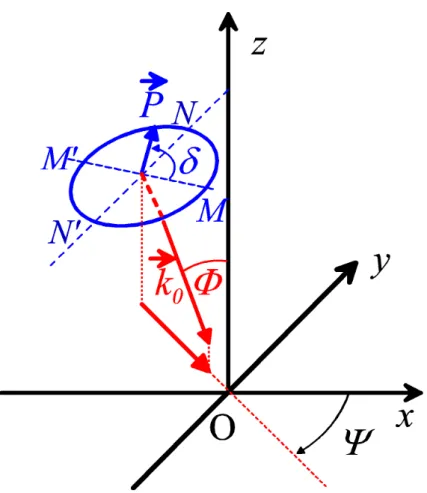
Now, we consider the diffraction problem schematized in figure 2.5. An incident wave of wavevector −→

k₀ is incident on a doubly-periodic structure separating air (region R0) from a grating material (region R1). We use all the notations defined in the preceding sections to characterize the materials. The incident field is schematized in figure 2.6. The direction of incidence is specified by the polar angles Φ andΨ (see figure 2.6). In order to define the polarization of the incident field, we construct the circle MNM’N’ in the plane perpendicular to

−

→k₀, with the continuation of NN’ intersecting thezaxis and MM’ being perpendicular to NN’.

The polarization angle δ is the angle between M’M and the direction of the incident electric field−→

P. With these notations, the incident electric field is given by:

−

→ Eⁱ=−→

Pexp iαx+iβy−iγz

, (2.92)

(25)

Figure 2.6: Notations for the incident field.

withα =k₀sinΦcosΨ, β =k₀sinΦsinΨ andγ =k₀cosΦ. The projection of−→

P on M’M is called transverse component of−→

P and denoted byP^t. Its projection on N’N is called longitudinal (in plane) component and denoted bzP^l, in such a way that−→

P =P^t

−−→MM⁰ MM⁰+P^l

−−→NN⁰ NN⁰.

As in the case of classical gratings, it is possible to show that above the top of the grating (z>z_M), the field can be expanded in the form of a sum of plane waves:

−

→E(x,z) =











∑^+∞_n=−∞∑^+∞_m=−∞

−−→I_0,n,mexp(iα_nx+iβ_my−iγ_0,n,mz)+

+−−−→

D_0,n,mexp(iα_nx+iβ_my+iγ_0,n,mz)

, ifz>z_M,

∑^+∞_n=−∞∑^+∞_m=−∞ −−−→

D_1,n,mexp(iα_nx+iβ_my−iγ_1,n,mz)+

+−−→

I_1,n,mexp(iα_nx+iβ_my+iγ_1,n,mz)

ifz<0.

(2.93)

The wavevectors of all these plane waves must be orthogonal to their vector amplitudes. As for the incident wave, we can define the transverse and longitudinal components of the vector amplitudes of the plane waves, the transverse component (for exampleD^t_0,n,m)being orthogonal to the z axis in the plane perpendicular to the wavevector (α_n,β_m,γ0,n,m) and the longitudinal (for exampleD^l_0,n,m)its component in the orthogonal direction of the same plane.

Using the Poynting theorem, it can be shown, as in section 2.5.3, that the efficiencies in thez-propagating orders are given by:

ρ_i,n,m=





 γ_0,n,m

γ0,0

|−→

D_0,n,m|² ifi=0,

γ_1,n,m γ0,0

( 1

ν²|D^l_1,n,m|²+|D^t_1,n,m|²) ifi=1.

(2.94)