A comparison with the Euler equations demonstrates the relevance of the Galilean invariance in the description of water waves. The aim of this paper is to investigate the relevance of the Galilean invariance in the description of water waves. The Galilean invariance (or Galilean relativity) is one of the fundamental properties of any mathematical model that originates in classical mechanics.
For a systematic study of the symmetries and the conservation laws of the full water wave formulation we have. To this end, in Section 3, solitary wave profiles of the new equations are generated numerically. In particular, the complete formulation of the water wave equations recognizes the Galilean boost symmetry and the invariance under the vertical translations (the latter issue will be addressed by the authors in a future work).
Specifically, unlike the KdV equation, the phase and group velocities of the BBM equation have a lower bound. We now present a modification of the classical BBM equation that allows us to restore the Galilean invariance property. As in the case of the Peregrine system, equations do not, as far as we know, have a Hamiltonian structure.
An integration of the mass conservation equation and the decay at infinity leads to u= csη.
The Serre equations
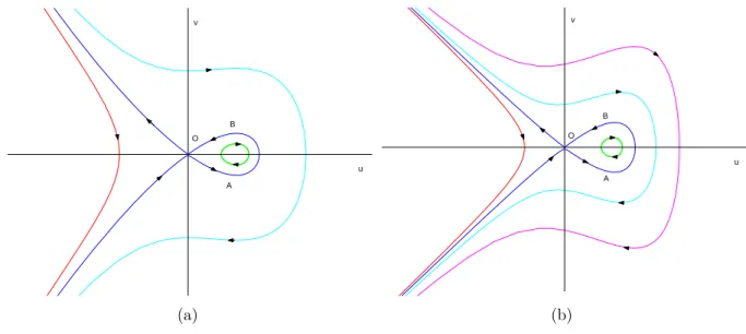
Similar to the case of iBBM, we can see that (2.25) is written as a first-order system and when c2s−gd >0, the origin is saddle; the phase plane sketched in Fig. 1(b) also shows a solitary wave in the form of an O →A→B →O trajectory.
Numerical computation of travelling waves
Computation of travelling-wave profiles. The Petviashvili method
Specifically, our implementation for the three systems has been performed by considering the corresponding periodic problem and using a pseudospectral representation for approximations to the profiles. As an initial approximation, a solitary wave solution (2.28) of the Serre equations or the third-order asymptotic solution of Grimshaw [37] can be considered. The iterative procedure is continued until the difference between two successive iterations in the L∞ norm, or the L∞ norm of the residual is less than a prescribed small tolerance, which in our case is of order O(10−15).
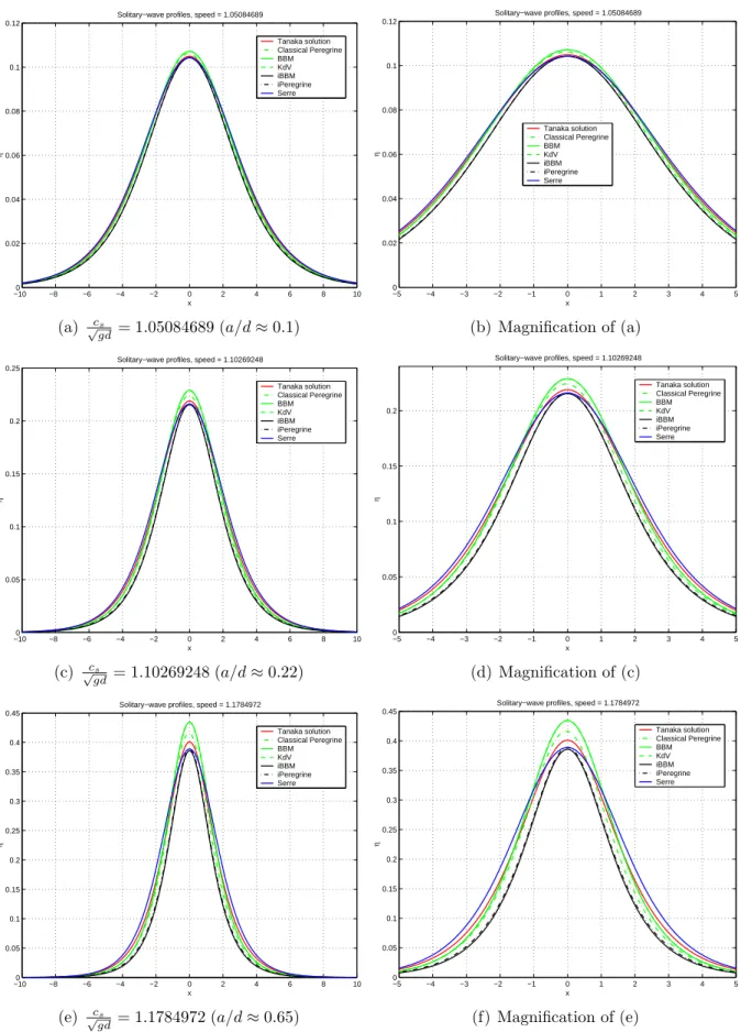
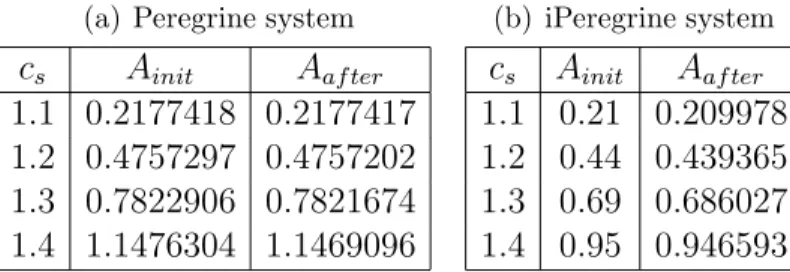
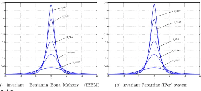
To better illustrate the transformations solitary waves undergo as we gradually increase the propagation speed parameter cs, we superimpose several profiles on the same figure (Figure 2(a) corresponds to the invariant Benjamin–Bona–Mahony (iBBM) system and Figure 2 ( b) to the immutable Peregrine (iPer) system). In order to determine the accuracy of the calculations, the three models considered in this paper were numerically integrated in time using the calculated solitary wave profiles as initial conditions. Some error indicators measuring the accuracy of the numerical approximation of the solitary waves were calculated.
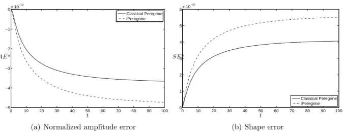
Some error indicators for the propagation of a solitaire for Peregrine and Peregrine invariant systems. We study the evolution of two parameters: the normalized amplitude error and the shape error. The first one is calculated by comparing, at each time step, the initial amplitude of the profile (created by the Petviashvili method) with the corresponding amplitude of the numerical solution calculated using the Newton method, [25].
The L2-based normalized shape error is also defined at each time step for, say, the solitary wave u as SEn = infτkUn−u(·, τ)k/ku(·,0)k. Figure 3(a) shows the temporal evolution of this amplitude error up to a final time T = 100, for both cPer and iPer. We observe that for the specific values of ∆x and ∆t the amplitude is preserved up to 10 decimal digits in both cases.
On the other hand, the shape error is calculated by comparing the numerical solution with time translations of the initial profile at a prescribed rate and minimizing the differences (see [26] for details). The results shown in Figure 3(b) show an almost constant evolution of this error, which in both cases is of the order of O(10-10). These results confirm the accuracy of the technique used to generate the solitary wave profiles and the numerical code for the time evolution.
Numerical results
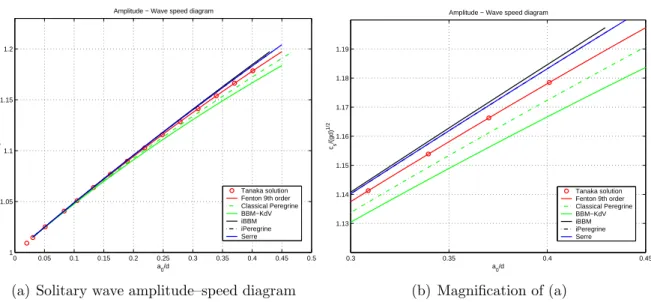
Tanaka solution Fenton 9th order Classic Peregrine BBM−KdV iBBM iPeregrine Serre. a) Solitary wave amplitude–velocity diagram. The curves corresponding to the iPeregrine system and the Serre system are superimposed up to the graphical resolution. The Tanaka solution is represented by red circles, while the Fenton solution is depicted by the red solid line.
According to these results, it is observed that the invariant Benjamin-Bona-Mahony (iBBM) equation and the invariant Peregrine (iPer) system approximate much better the amplitude of the reference solution (in this case represented by Tanaka's solution) than the non-Galilean invariants counterparts, and they stay very close to the results of the Serre system near the top. As a measure of the level of approximation to solitary wave solutions of the Euler system, these and the previous results show the advantages of taking into account the invariantization process in the approximated models.
Solitary waves dynamics
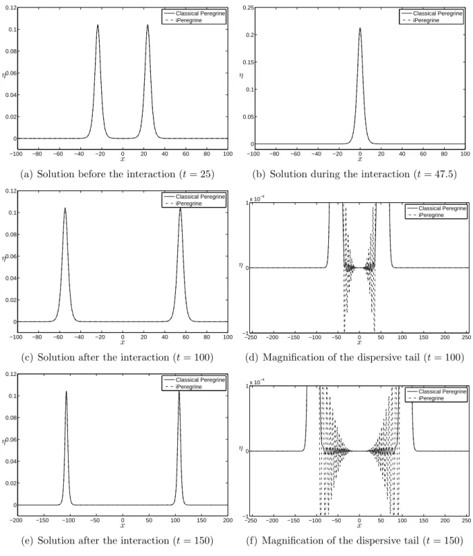
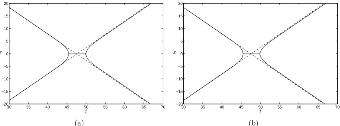
- Head-on collisions of solitary waves
- Overtaking interactions of solitary waves
- Comparison with laboratory data
- Comparison with Euler equations
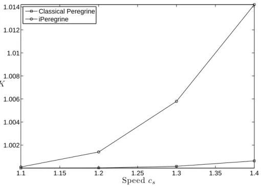
Then a ratio K of the amplitude of the waves after the collision to their amplitude before the collision is calculated. Figure 6 shows the behavior of this value as a function of speed parameters and for both systems. The results reveal a higher inelastic collision in the case of the invariant system, consistent with that observed in the full water wave model [21].
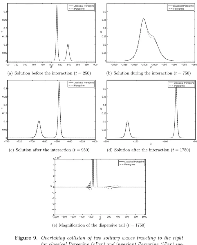
In figure 9 we observe that the basic characteristics of the interaction are the same for both systems (see also [2]). Furthermore, a small phase shift and a shape change can be observed in the solitary pulses (Figure 8). The wavelet generated in the case of the classical Peregrine system has an inverse N-shape, while the invariant version has an N-shape.
With the same input data, Figure 10at shows the overtaking collision for the case of the BBM and iBBM equations several times. The phase shift observed in the iBBM case is also larger, again indicating a larger amount of nonlinearity and inelasticity in the specific interaction. We can conclude that these two groups of results show that, as expected, the O(εµ2) nonlinear terms of invariant models do not significantly change the behavior of solitary wave interactions provided by the corresponding non-Galilean invariant system in a qualitative sense.
To answer this question, we compare the numerical solution of the cPer and iPer systems during a head-on collision with some experimental data from [21]. A closer look at the dispersive tails shows that again after their interaction a pantry dispersive tail is generated in the case of the iPer system. Finally, we study the evolution of a solitary wave of the Euler equations when we use it as an initial condition for the approximate models.
Catch-up collision of two right-moving solitary waves for classical Peregrine (cPer) and invariant Peregrine (iPer) systems. In the case of the Peregrine and the iPeregrine systems we use for initial velocity u0(x) =csη0(x)/d+η0(x). Evolution of a solitary wave of the Euler equations, with BBM, iBBM, cPer and iPer models.
Figure 13(a) shows the shape error of the solution (i.e. how much the solution differs from being the exact solitary wave of the Euler equations), while Figure 13(b) shows the amplitude of the solution as a function of time t. From these two figures, we observe that in the case of classical models, the emergent solitary waves are closer in shape and amplitude to the original solitary wave solution of the Euler equations than the respective solitary waves of the invariant models.
Conclusions
Kinematics and stability of solitary and cnoidal wave solutions of the Serre equations.Eur. A numerical study of the stability of solitary waves of the Bona-Smith family of Boussinesq systems.J. On the change of form of long waves advancing in a rectangular channel, and on a new type of long stationary waves.Phil.
A generalized Petviashvili iteration method for scalar and vector Hamiltonian equations with arbitrary form of nonlinearity.J. A numerical study of the exact evolution equations for surface waves in water of finite depth. Stud.