HAL Id: tel-00924445
https://tel.archives-ouvertes.fr/tel-00924445
Submitted on 6 Jan 2014
HAL is a multi-disciplinary open access archive for the deposit and dissemination of sci- entific research documents, whether they are pub- lished or not. The documents may come from teaching and research institutions in France or abroad, or from public or private research centers.
L’archive ouverte pluridisciplinaire HAL, est destinée au dépôt et à la diffusion de documents scientifiques de niveau recherche, publiés ou non, émanant des établissements d’enseignement et de recherche français ou étrangers, des laboratoires publics ou privés.
Approches de programmation par contraintes pour l’analyse des propriétés structurelles des réseaux de
Petri et application aux réseaux biochimiques
Faten Nabli
To cite this version:
Faten Nabli. Approches de programmation par contraintes pour l’analyse des propriétés structurelles des réseaux de Petri et application aux réseaux biochimiques. Bioinformatics [q-bio.QM]. Université Paris-Diderot - Paris VII, 2013. English. �tel-00924445�
THESE
Présentée pour obtenir le titre de
DOCTEUR DE L’UNIVERSITE PARIS DIDEROT Spécialté: Informatique
Par
Faten Nabli
Approches de programmation par contraintes pour l’analyse des propriétés structurelles des réseaux de
Petri et application aux réseaux biochimiques
Présentée le 10 juillet 2013 devant le jury composé de :
Rapporteurs: Prof. Alexander Bockmayr - Freie Universität Berlin Prof. Karsten Wolf - Universität Rostock
Superviseurs: Prof. François Fages - INRIA Paris-Rocquencourt Dr. Sylvain Soliman - INRIA Paris-Rocquencourt Président: Prof. Michel Habib - Université Paris Diderot- Paris7 Examinateurs: Prof. Hanna Klaudel - Université d’Evry
Dr. Sabine Peres - Université Paris-Sud
Invités : -
Contents
List of Figures vi
List of Tables vii
1 Petri Nets 9
1.1 Definitions . . . 10
1.2 Structural Properties . . . 13
1.2.1 Place/Transition invariants . . . 13
1.2.2 Siphons and Traps . . . 14
1.2.3 Known Time Complexity Of Minimal Siphon Extraction Prob- lem . . . 18
1.3 New Time Complexity Result . . . 22
1.3.1 Polynomial time complexity theorem for Petri-nets with bounded tree-width . . . 22
1.3.2 Linear Time Complexity Result . . . 27
1.4 Petri Net Structures and CTL Properties . . . 29
1.4.1 Infinite State Computation Tree Logic . . . 29
1.4.2 Boolean Abstractions, Boundedness Conditions and Boolean CTL Model-Checking . . . 34
2 Petri Nets for Biochemical Networks 41 2.1 Biological context . . . 42
2.1.1 Systems Biology . . . 42
2.1.2 Molecular Biology and Cellular Metabolism . . . 42
2.1.3 Biochemical Networks . . . 43
2.2 Biochemical Networks modelling . . . 46
2.2.1 Boolean and Discrete modelling . . . 46
2.2.2 Continuous and stochastic Modelling . . . 46
2.2.3 Petri nets modelling of biochemical networks . . . 47
2.3 Benchmark . . . 50
2.3.1 Biomodels.net . . . 50
2.3.2 Petriweb . . . 51
2.4 Petri net properties on the benchmark . . . 52
2.4.1 P-invariants as mass conservation laws . . . 52
2.4.2 T-invariants as flux conservation . . . 52
2.4.3 Siphons/Traps . . . 53
3 Boolean Model for siphons/traps 55 3.1 Constraint Programming (CP) and Systems Biology . . . 55
3.2 Boolean Model . . . 56
3.3 Boolean Algorithms . . . 58
3.3.1 Iterated SAT Algorithm . . . 58
3.3.2 Backtrack Replay CLP(B) Algorithm . . . 60
3.4 Evaluation . . . 61
3.4.1 Results and Comparison . . . 61
3.4.2 Hard instances . . . 62
3.5 CLP model for the Siphon-Trap Property (STP) . . . 66
4 Constraint Programming Approach to P/T invariants 69 4.1 P/T-invariants Computation . . . 70
4.1.1 The Fourier-Motzkin Algorithm for P/T-invariants . . . 70
4.1.2 Finding P/T-invariants as a Constraint Solving Problem . . . 73
4.1.3 Symmetry detection and elimination . . . 75
4.1.4 Experimental Results . . . 76
4.2 Steady-state solution of biochemical systems, beyond S-Systems via T-invariants . . . 77
4.2.1 Biochemical Systems Theory . . . 77
4.2.2 Method . . . 79
4.2.3 Results . . . 84 4.2.4 Conclusions and Perspectives . . . 90
A Appendix 1 95
General Conclusion 95
Bibliography 99
List of Figures
1.1 A Petri net with an arbitrary marking enabling t3 . . . 11
1.2 Petri net of Figure 1.1 after the firing of t3 . . . 11
1.3 Petri net graph of Example 5. . . 15
1.4 Petri net for reduction of 3-SAT problem of example 7: for i = 1,2,3,4, ri and r¯i, si and s¯i, yi and y¯i correspond to literals, re- spectively variables and their negation. for i= 1,2,3, ui correspond to clauses. . . 19
1.5 Graph example (G) with 6 vertices . . . 23
1.6 Cut-width of G for a numbering l . . . 23
1.7 Tree decomposition G . . . 24
1.8 Hyper-graph example H . . . 24
1.9 Primal graph of H . . . 24
1.10 Petri net depicting the enzymatic reaction . . . 25
1.11 Hyper-graph of the Petri net depicted in Figure 1.10 . . . 25
1.12 Primal graph of the Petri net depicted in Figure 1.10 . . . 25
1.13 Primal graph of CSP(N) . . . 26
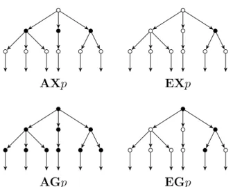
1.14 Reachability trees for AXp, EXp, AGp, and EGp. . . 30
1.15 An example of Kripke structure . . . 31
2.1 Information flow from genes to metabolites in cells . . . 43
2.2 Map of yeast protein-protein interactions . . . 44
2.3 Petri net modelling a part of the glycolysis and the pentose phosphate pathway in erythrocytes . . . 45
2.4 Conceptual Framework. The Petri net formalism allows to switch between different network classes to describe standard (qualitative) Petri nets, stochastic (SPN) and continuous (CPN) information in a cohesive Petri net model [47]. . . 48
2.5 Petri-net graph modelling the growth metabolism of the potato plant [107]. . . 53 3.1 Search tree developed with the backtrack replay strategy for enumer-
ating the 64 minimal siphons of model 239 of biomodels.net (described in Section 2.3). Each red end corresponds to a minimal siphon found.
Very few backtracks are necessary thanks to the constraint propaga- tion and the strategy . . . 61 3.2 Computation time random 3-SAT . . . 63 3.3 Probability of random 3-SAT satisfiablity . . . 64 3.4 Distribution of density of 3-SAT models derived from Biomodels.net.
Computed tree-widths are less or equal than 10. . . 65 3.5 Variation of tree-width as a function of size (places and transitions)
on Petri nets of Biomodels.net . . . 66 3.6 Petri net modelling the problem of 2 dining philosophers . . . 68 4.1 A Petri net example for Fourier-Motzkin algorithm . . . 71 4.2 A diagram describing the model 9 of the Biomodels.net repository. . . 86
List of Tables
3.1 Computation time in milliseconds on the biomodels and Petriweb benchmarks. . . 61 3.2 Computation time in milliseconds on the hardest instances of bio-
chemical networks. . . 62 3.3 Tree-width of the hardest instances of Biomodels.net database. . . 66 3.4 Siphon-Trap Property evaluation on k dining philosophers Petri nets . 68
Abstract
Petri nets are a simple formalism for modelling concurrent computation. This for- malism has been proposed as a promising tool to describe and analyse biochemical networks. In this thesis, we explore the structural properties of Petri nets as a mean to provide information about the biochemical system evolution and its dynamics, especially when kinetic data are missing, making simulations impossible.
In particular, we consider the structural properties of siphons and traps. We show that these structures entail a family of particular stability properties which can be characterized by a fragment of CTL over infinite state structures. Mixed integer linear programs have been proposed and a state-of-the-art algorithm from the Petri net community has been described later to compute minimal sets of siphons and traps in Petri nets. We present a simple boolean model capturing these notions and compare SAT and CLP methods for enumerating the set of all minimal siphons and traps of a Petri net. Our methods successfully apply to a practical benchmark composed of the 404 models from the biomodels.net repository. We analyse why these programs perform so well on even very large biological models although the decision problem is NP-complete. We show that, in networks with bounded tree- width, the existence of a minimal siphon containing a given set of places can be decided in linear time, and the Siphon-Trap property as well.
Moreover, we consider two other Petri net structural properties: place and tran- sition invariants. We present a simple method to extract minimal semi-positive invariants of a Petri net as a constraint satisfaction problem on finite domains using constraint programming with symmetry detection and breaking. This allows us to generalize well-known results about the steady-state analysis of symbolic Ordinary Differential Equations systems corresponding to biochemical reactions by taking into account the structure of the reaction network. The study of the underlying Petri net, initially introduced for metabolic flux analysis, provides classes of reaction systems for which the symbolic computation of steady states is possible.
General Introduction
Systems Biology
The development of high-throughput data collecting techniques, for example, micro- arrays, protein chips, yeast two-hybrid screens, etc., are used in systems biology to create databases, interaction maps and detailed models of complex reaction sys- tems at the cellular level. As examples of large models that emerged over the past few decades, we can cite the biggest MOOSE (multi-scale) model [32] with about 7500 species and 10000 reactions; a large structural yeast model with 2153 species (1168 metabolites, 832 genes, 888 proteins and 96 catalytic protein complexes) and 1857 reactions (1761 metabolic reactions and 96 complex formation reactions); the RB/E2F map established by Curie Institute [10], with 530 reactions and 390 species, and being currently merged with the EGFR map of the Systems Biology Institute [82] with its 219 reactions and 322 species.
To facilitate exchange of such models, standard formats for encoding quanti- tative information have been developed. As examples of such formats, we find CellML (www.cellml.org) and NeuroML (www.neuroml.org), but the Systems Bi- ology Markup Language (SBML) [54] has so far been the most successful standard model exchange format in this field. It has been adopted by more than 180 software systems ranging from simulators to model editors and databases.
It is also crucial to classify this enormous amount of models into databases where models can be freely deposited and distributed in standardised for- mats. New databases for systems biology appeared like the Reactome database (www.reactome.org) that contains curated models of core pathways and reactions in human biology. EcoCyc (www.ecocyc.org) and MetaCyc (wwww.metacyc.org) are databases of non redundant, experimentally elucidated metabolic pathways. EcoCyc contains data modelling metabolic pathways of the bacterium Escherichia coli K-12 MG1655. MetaCyc covers data from different organisms. It contains more than 1928 pathways from more than 2263 different organisms, and is curated from the scientific experimental literature. Biomodels.net (www.biomodels.net) database has also be- come a recognised reference repository for systems biology. It is a freely-accessible on line resource for storing, viewing, retrieving, and analysing published, peer-reviewed quantitative models of biochemical and cellular systems.
Simulation is currently the primary use of these models and the structure and
behaviour of each simulation model distributed by Biomodels.net database are thor- oughly checked; in addition, model elements are annotated with terms from con- trolled vocabularies as well as linked to relevant data resources. Models can be examined on line or downloaded in various formats. Reaction network diagrams generated from the models are also available in several formats. Biomodels.net database also provides features such as on line simulation and the extraction of components from large scale models into smaller sub-models. Finally, the system provides a range of web services that external software systems can use to access up-to-date data from the database.
Having biochemical models and filling them with experimental data was the first challenge of biologists. With the increase of available information, the challenge of efficient information processing is arising: especially when kinetic parameters are lacking which make simulations not possible without guessing them. In some cases, the model structure may however be detailed enough to provide some useful information about the dynamics.
Petri nets
Petri nets are a simple formalism for modelling concurrent computation. Petri nets provide a tool to model biochemical reaction networks and provide powerful qual- itative and quantitative analysis techniques. The intuitive description of chemical process coupled with the possibility to simulate and analyse token movement, repre- senting substance or information flow in biochemical systems, facilitates the use of Petri net in systems biology. The motivation for using Petri nets to model biochem- ical networks comes mainly from the fact that biochemical systems exhibit many concurrent reactions, similar to concurrent process in technical systems. In 1993, Reddy et al. introduced a method of representation of metabolic pathways as Petri nets, and illustrate some useful properties like liveness, reachability, reversibility fairness and invariants [85]. Then in 1994, Hofestadt [50] described the metabolic process depending on expressed genes as Petri nets. Moreover, Petri nets are also suitable to model medical systems because of the lack of experimental data due to experiments difficulties and ethical reasons. Since 1993, many applications have been published and Petri nets have been applied to many biochemical examples such as metabolic systems [50, 85, 107] gene regulatory networks [72, 73], signal trans- duction networks [73, 89] the glycolysis and pentose phosphate pathway and the carbon metabolism in Tuber. Different types of Petri nets extension have been used to model and analyse biochemical networks, going from coloured Petri nets, hybrid Petri nets [72, 73], continuous Petri nets[51] and stochastic Petri nets.
Thesis contribution
In this thesis, we focus on Petri nets structural properties and how they can be computed using constraint programming techniques. The structural properties of interest give us some information about the biochemical reaction network and its dynamics, even when there is a lack in kinetic data making simulation impossible.
As application, we evaluate them on the Biomodels.net database.
We consider the Petri net concepts of siphons and traps. A siphon is a set of places that, once it is unmarked, remains so. A trap is a set of places that, once it is marked, can never loose all its tokens. Thus, siphons and traps have opposing effects on the token distribution in a Petri net. These structural properties provide sufficient conditions for reachability (whether the system can reach a given state) and liveness (freedom of deadlocks) properties. It is proved that in order to be live, it is necessary that each siphon remains marked. Otherwise (i.e. once it is empty), transitions having their input places in a siphon can not be live. One way to keep each siphon marked is to have a marked trap inside it. In fact, this condition is necessary and sufficient for a free-choice net to be live [83]. Siphons can correspond to a set of metabolites that are gradually reduced during starvation whereas traps can correspond to accumulation of metabolites that are produced during the growth of an organism. It has been shown that finding a minimal siphon of a given cardinality or even containing a given set of places is NP-complete [101, 106]. Mixed integer linear programs have been proposed in [78, 21] and a state-of-the-art algorithm from the Petri net community has been described later in [23] to compute sets of minimal siphons and traps in Petri nets. We present a simple Boolean model capturing these notions and two methods for enumerating the set of all minimal siphons and traps of a Petri net. The first method iterates the resolution of the Boolean model executed with a SAT solver. The second method proceeds by backtracking with a CLP(B) program. On a benchmark composed of the 80 Petri nets of Petriweb1 [45] and the 404 curated biological models of the biomodels.net2 repository [66], we show that miniSAT and CLP(B) solvers are both faster by two orders of magnitude than the dedicated algorithms and can in fact solve all instances.
Furthermore, we analyse why these programs perform so well even on very large biological models. We show that in networks with bounded tree-width, the existence of a minimal siphon containing a given set of places can be decided in linear time [80]. We show also that deciding the Siphon-Trap property can be done in linear time in networks with bounded tree-width.
Moreover, we show that siphons and traps entail a family of particular stability properties which can be characterized by a fragment of CTL over infinite state structures. Interestingly, we show that a well-founded Boolean abstraction of the Petri net preserves a similar characterization of Boolean CTL properties as siphons and traps. This fragment of boolean CTL formulas can thus be verified without recourse to symbolic model-checking methods by a purely structural analysis of the
1http://www.petriweb.org/
2http://www.biomodels.net/
Petri net.
We also consider the Petri net structural properties of place and transition in- variants. A P-invariant stands for a set of places over which the weighted some of tokens is constant and independent of any firing. P-invariants correspond to conser- vation law. On the other hand, a T-invariant has actually two interpretations in the given biochemical network: first, the entries of a T-invariant represent a multi-set of transitions, which reproduce a given marking by their partially ordered firing. That means that they occur basically one after the other. The partial order sequence of the firing events of the T-invariant’s transitions may contribute to a deeper under- standing of the system behaviour. Second, the entries of a T-invariant may also be read as the relative firing rates of transitions, all of them occurring permanently and concurrently. This activity level corresponds to the steady state behaviour and min- imal T-invariants correspond to elementary modes classically studied for metabolic networks.
We present a simple method to extract minimal semi-positive invariants of a Petri net modelling a biological reaction system, as a constraint satisfaction problem on finite domains using constraint programming with symmetry detection and breaking.
An implementation based on GNU-Prolog’s FD solver of the method is incorporated in the BIOCHAM modelling environment [9, 35]. Two prototypes for computing minimal P-invariants and minimal T-invariants are evaluated on our benchmark of interest. Moreover, we present a way to generalize well-known results about the steady-state analysis of some symbolic Ordinary Differential Equations systems by taking into account the structure of the reaction network. The structural study of the underlying Petri net, usually used mostly for metabolic flux analysis, provides classes where the computation of some steady states of the system is possible, even though the original symbolic model did not form an S-system and was not solvable by state-of-the-art symbolic computation software.
Roadmap
The manuscript is organized as follows. In the first chapter we focus on the Petri net formalism. We define notions and notations that are necessary for the understanding of the following work. We prove a new linear complexity result for the siphon extraction problem in Petri nets of bounded tree-width. We develop links between the structural properties of siphons and traps and their dynamical properties in Computation Tree Logic.
In the second chapter, we present the biological background, here we recall the concepts of molecular biology and we enlarge our definition of biochemical networks.
In the third chapter, we describe a boolean model for the problem of enumerating all minimal siphons in a Petri net and we compare two boolean methods to a state- of-the-art algorithm from the Petri net community [23].
In the last chapter, we introduce a new method based on Finite Domain con-
straint programming to efficiently compute place and transition invariants of a re- action network. It includes symmetry detection and breaking and scales up well to the biggest reaction networks found. We present also a new method to compute, in a fully analytical way, steady states of biochemical systems defined by a system of Ordinary Differential equations.
Finally, we conclude this manuscript with a summary and an outlook on future work.
Chapter 1 Petri Nets
Contents
1.1 Definitions . . . 10
1.2 Structural Properties . . . 13
1.2.1 Place/Transition invariants . . . 13
1.2.2 Siphons and Traps . . . 14
1.2.3 Known Time Complexity Of Minimal Siphon Extraction Problem . . . 18
1.3 New Time Complexity Result . . . 22
1.3.1 Polynomial time complexity theorem for Petri-nets with bounded tree-width . . . 22
1.3.2 Linear Time Complexity Result . . . 27
1.4 Petri Net Structures and CTL Properties . . . 29
1.4.1 Infinite State Computation Tree Logic . . . 29
1.4.2 Boolean Abstractions, Boundedness Conditions and Boolean CTL Model-Checking . . . 34
Introduction
Petri nets have been introduced in 1962 by Carl Adam Petri in his dissertation.
Petri nets are a mathematical modelling tool for describing and analysing systems characterized as being concurrent, parallel, distributed and/or stochastic. Since their early introduction, Petri nets and their concepts have been extended and de- veloped, and applied in a variety of areas such as office automation, work-flows, flexible manufacturing, protocols and networks, real-time systems, embedded sys- tems, telecommunications, Internet, e-commerce, trading and biological systems.
1.1 Definitions
A Petri net or place/transition net is a directed bipartite graph, in which the nodes represent transitions (i.e. events that may occur, graphically represented by rectan- gles) and places (i.e. conditions, graphically represented by circles). The directed arcs are allowed to connect only nodes from different classes. The dynamics of a Petri net is obtained by moving the tokens in the places (graphically represented by bullets inside places). A directed arc represents conditions to fire transitions.
Formal definitions and basic terminology is presented in this section.
Definition 1 (Petri net graph). A Petri net graph is a weighted bipartite directed graph P N = (P, T, W), whereP is a finite set of vertices called places, T is a finite set of vertices (disjoint from P) called transitions andW : ((P×T)∪(T×P))→N represents a weight function attached to the arcs.
The weight is represented by an integer located near the arc. If this integer is missing, it is assumed that the weight of the arc is 1 (the weight zero represents the absence of arc).
Definition 2 (Marking). Amarking for a Petri net graph is a mappingm :P →N which assigns a number of tokens to each place. We say that a place p is marked if and only if m(p)>0, otherwise, it is said to be unmarked.
Definition 3 (Petri net). A Petri net is a 4-tuple (P, T, W, m0) where (P, T, W) is a Petri net graph and m0 is an initial marking.
Definition 4 (Predecessors/successors). The set of predecessors (resp. successors) of a transition t ∈ T is the set of places •t = {p ∈ P | W(p, t) > 0} (resp. t• = {p ∈ P | W(t, p) > 0}). Similarly, the set of predecessors (resp. successors) of a place p∈P is the set of transitions •p={t ∈T |W(t, p)>0} (resp. p• ={t ∈T | W(p, t)>0}).
The set of predecessors (resp. successors)•S (resp. S•) of a set of placesS is the union of sets of predecessors (resp. successors) of each place p ∈ S: •S = S
p∈S•p (resp. S• =S
p∈Sp•).
The set of predecessors (resp. successors) •Q (resp. Q•) of a set of transitions Q is the union of sets of predecessors (resp. successors) of each transition t ∈ Q:
•Q=S
t∈Q•t (resp. Q• =S
t∈Qt•).
Definition 5 (Transition enabling and firing). For every two markings m, m′ :P → N and every transition t ∈ T, there is a transition step m →t m′, if for all p ∈ P, m(p) ≥ W(p, t) and m′(p) = m(p)−W(p, t) + W(t, p). A transition t is enabled at marking m, (m →) if and only ift ∀p ∈ •t : m(p) ≥ W(p, t). m →t m′ means that the transition t is enabled in m and its firing leads to m′. m′ is such that
∀p ∈ P, m′(p) = m(p)−W(p, t) +W(t, p). An enabled transition may or may not fire (depending on whether or not the corresponding event actually takes place).
Definition 6(Firing sequence).A finite sequence of transitionsσ = (t0. . . tn)is a fi- nite firing sequence of the Petri net if there exists a sequence of markingsm1, . . . , mn
for which m→t0 m1 t1
→. . .tn−→1 mn tn
→m′. This is denoted as m→σ m′.
p1 p2
p3
p4
t1 2 t2
4
t3
t4
2 2
Figure 1.1: A Petri net with an arbitrary marking enabling t3
Example 1. In the Petri net depicted in Figure 1.1 , starting from a marking with 3 tokens in p1 and 2 tokens in p4, one can remove two tokens from p1 to produce 4 tokens in p2 (firing of t2) and one can remove one token from p1 and 2 tokens of p4 and produce one token in p3 (firing of t3). And then remove one token from p2 and one token from p3 to produce two tokens in p4 (firing of t4). From this initial marking, firing justt3 leads to the Petri net of Figure 1.2. Petri nets can intuitively model metabolic reactions by corresponding places to metabolites and transitions to reactions. Tokens inside places represent the number of molecules or the level of concentration of species. In the next chapter, we provide some examples of Petri nets modelling biochemical networks.
p1 p2
p3
p4
t1 2 t2
4
t3
t4
2 2
Figure 1.2: Petri net of Figure 1.1 after the firing oft3
Definition 7 (Incidence Matrix). Let P = (p1, p2, ..., pn) (resp. T = (t1, t2, ..., tm)) be the set of places (resp. transitions) of a Petri net. The incidence matrix of this Petri net is A= [aij], i= 1, ..., n;j = 1, ...m defined as follows:
aij =W(pi, tj)−W(tj, pi)
Example 2. The Petri net of figure 1.1 has the following incidence matrix:
t1 t2 t3 t4
p1 1 −2 −1 0
p2 0 4 0 −1
p3 0 0 1 −1
p4 0 0 −2 2
The second column of this matrix can be read as: the firing of t2 removes two tokens from p1 and produces four tokens in p2.
Definition 8 (Firing count vector). A vectorσ¯ is the firing count vector of σ ifσ(t)¯ equals the number of times transition t occurs in the firing sequence σ.
Definition 9 (Behaviour properties). Let N = (P, T, W, m0) be a Petri net
• A place p is k-bounded if there is a positive integer number k such that the number of tokens in p does never exceed k.
• A Petri net is k-bounded if all its places are k-bounded.
• A transition t is dead at marking m if it is not enabled in any marking m′ reachable from m.
• A transition t is live if it is not dead in any marking reachable from m0.
• A marking m is dead if there is no transition enabled in m.
• A Petri net is deadlock free (weakly live) if there is no reachable dead markings.
• A Petri net is live (strongly live) if each transition is live.
Definition 10 (Net Structures). Let N = (P, T, W) a Petri net graph. N is
• Homogeneous if ∀p∈P :t, t′ ∈p• ⇒W(p, t) = W(p, t′).
• Ordinary if ∀p∈P and ∀t ∈T, W(p, t)≤1 and W(t, p)≤1.
• Extended simple (or asymmetric choice) if it is ordinary and
∀p, q ∈P :p•∪q• =∅ ∨p• ⊆q•∨q• ⊆p•.
• Extended free choice if it is ordinary and
∀p, q ∈P :p•∩q• =∅ ∨p• =q•.
1.2 Structural Properties
Various dynamical properties of Petri nets can be verified by constructing the reach- ability graph and analysing it. However, the reachability graph is generally infinite.
In fact, the reachability problem was shown to be EXPSPACE-hard [68] years be- fore it was shown to be decidable [74]. Structural analysis makes it possible to prove some properties without constructing the reachability graph. Structural properties do not depend on any marking: they depend only on the topology of the Petri net graph.
1.2.1 Place/Transition invariants
A place invariant is a set of places, whose weighted sum of tokens is constant inde- pendently of the sequence of firing. A transition invariant is a potential firing set without any net effect.
Definition 11 (P-invariant). A vector V = [v1, v2, ..., vn] with non-negative integer components is a P-invariant ifV 6= 0 and V A= 0, where A is the incidence matrix of the Petri net with n places and m transitions.
Example 3. A P-invariant of the Petri net represented in figure 1.1 is such that:
[v1, v2, v3, v4]
1 −2 −1 0 0 4 0 −1 0 0 1 −1 0 0 −2 2
=
0 0 0 0
which leads to:
v1 = 0
−2v1+ 4v2 = 0
−v1 +v3−2v4 = 0
−v2 −v3+ 2v4 = 0
Thus any vector V = [0,0,2k, k], where k is a non-negative integer is a p- invariant.
Proposition 1. [83] If V is a P-invariant and m0 is an initial marking of a Petri net, V mt0 =V mt for any m reachable from m0.
For instance, in the previous example, 2m(p3) +m(p4) is constant whatever m is.
Definition 12 (T-invariant). A vector Y = [y1, ...ym] with non-negative integer components is a T-invariant if AYt = 0, where A is the incidence matrix of the Petri net with n places and m transitions.
Example 4. A t-invariant of a Petri net represented in figure 1 is such that:
1 −2 −1 0 0 4 0 −1 0 0 1 −1 0 0 −2 2
y1
y2
y3 y4
=
0 0 0 0
which leads to:
y1−2y2 −y3 = 0 4y2 −y4 = 0 y3−y4 = 0
−2y3+ 2y4 = 0
Hence, any vector Y = [6k, k,4k,4k], where k is a non-negative integer is a t- invariant.
Proposition 2. [83] Let σ be a firing sequence and Vσ be the counting vector of σ.
Let m be the marking reached by firing σ. IfVσ is a T-invariant, then m=m0. Definition 13 (Support). The support of a P-invariant x or a T-invarianty is the set of places or transitions respectively corresponding to the strictly positive compo- nents ofxandy, and are denoted by||x||and||y||, i.e.,||x||={p∈P |x(p)>0}
and ||y||={t∈T |y(t)>0}.
Definition 14 (Minimal invariant). A P-invariant is minimal if no non-empty sub- set of the support is the support of some other P-invariant, i.e., x is a minimal P-invariant if there is no other P-invariant x′ such that x′(p)≤x(p) for all p, and the greatest common divisor of all entries of x is 1.
A T-invariant is minimal if no non-empty subset of the support is the support of some other T-invariant, i.e., y is a minimal T-invariant if there is no other T- invariant y′ such that y′(t) ≤ y(t) for all t, and the greatest common divisor of all entries of y is 1.
1.2.2 Siphons and Traps
A siphon is a set of places that once unmarked remains so whereas a trap is a set of places that once marked remains so. We recall that a set of places S is marked if at least one place p inS holds some tokens. Formal definitions are presented in the following. Let P N = (P, T, W) be a Petri net graph.
Definition 15. A trap is a non-empty set of places P′ ⊆ P whose successors are also predecessors: P′• ⊆•P′.
A siphon is a non-empty set of places P′ ⊆ P whose predecessors are also suc- cessors: •P′ ⊆P′•.
A siphon (resp. trap) is proper if its predecessors set is strictly included in its successors set,•P′ (P′•.
A siphon (resp. a trap) is minimal if it does not contain any other siphon (resp. trap).
It is worth remarking that a siphon in a Petri net graph P N is a trap in the dual Petri net graph, obtained by reversing the direction of all arcs in P N. Note also that since predecessors and successors of an union are the union of predecessors (resp. successors), the union of two siphons (resp. traps) is a siphon (resp. a trap).
Example 5. In the Petri net graph depicted in Figure 1.3, {A, B} is a minimal proper siphon: •{A, B} = {r1, r2} ⊂ {A, B}• = {r1, r2, r3}. {C, D} is a minimal proper trap: {C, D}• ={r4, r5} ⊂•{C, D}={r3, r4, r5}.
The following propositions show that traps and siphons provide a structural characterization of some particular dynamical properties on markings.
Proposition 3. [83] For every subset P′ ⊆ P of places, P′ is a trap if and only if for any marking m ∈ NP with mp ≥ 1 for some place p ∈ P′, and any marking m′ ∈NP such that m →σ m′ for some sequence σ of transitions, there exists a place p′ ∈P′ such that m′p′ ≥1.
Proposition 4. [83] For every subsetP′ ⊆P of places, P′ is a siphon if and only if for any markingm∈NP withmp = 0 for allp∈P′, and any marking m′ ∈NP such that m→σ m′ for some sequence σ of transitions, we have m′p′ = 0 for all p′ ∈P′.
A B C D
r1
r2
r3
r4
r5
Figure 1.3: Petri net graph of Example 5.
Although siphons and traps are stable by union, it is worth noting that minimal siphons do not form a generating set of all siphons. A siphon is called a basis siphon if it can not be represented as a union of other siphons [78]. Obviously, a minimal siphon is also a basis siphon, however, not all basis siphons are minimal.
For instance, in Example 5, there are two basis siphons, {A, B} and {A, B, C, D}, but only the former is minimal, the latter cannot be obtained by union of minimal siphons.
Minimal Siphons and strong connectedness
In this part, we show that the set of places forming a minimal siphon (in term of inclusion) form a strongly connected subnet.
Definition 16 (Strongly connected Petri net). A Petri net is strongly connected when for every pair of nodes (i.e., places and transitions) x and y, there exists a path leading from x to y.
Definition 17 (Subnet). Let G=(P, T, F) be a Petri net. P˜ ⊆ P and T˜ ⊆ T. Then G˜ = ( ˜P ,T ,˜ F˜) is the subnet of G generated by P˜ ∪T˜ iff F˜(p, t) = F(p, t), F˜(t, p) =F(t, p) ∀p∈P ,˜ ∀t ∈T˜.
Example 6. The Petri net G(P, T, F) is shown on figure on the left. The subnet generated by {A, B, D} ∪T is shown on figure on the right.
A B
C D
t1 t2
t3
t4
A B
D
t1 t2
t3
t4
Proposition 5. Let S be a minimal siphon in a Petri net N. The subnet NS
generated by S∪•S is strongly connected.
Proof. First we remark that every transition t of NS is a predecessor of some place of NS by definition of NS and also a successor of some place of NS since S is a siphon. Hence, for proving thatNS is strongly connected, we need just to show that for every two places x and y, there is a path between xand y inNS. Let y∈S and let the set X = {z ∈ S | there is a path leading from z to y in NS}. It suffices to show that X = S. For every transition t ∈ •y, there exists some y′ in S such that t ∈y′•. Hence there exists a path leading from y′ toy. and•t∩S ⊆X and•X ⊆X• then X is a non empty siphon included in S. Since S is minimal then X=S.
Application to the Siphon-Trap property
The concepts of live Petri nets (no dead transition) and especially of deadlock free Petri nets are important. A deadlock occurs if no transitions can be fired any longer.
This corresponds to a system which is either badly designed or badly modelled. One reason to consider minimal siphons is that they provide a sufficient condition for the non-existence of deadlocks. It has been shown indeed that in a deadlocked Petri net (i.e. where no transition can fire), all unmarked places form a siphon [16]. The siphon-based approach for deadlocks detection checks if the net contains a proper siphon that can become unmarked by some firing sequence. A proper siphon does not become unmarked if it contains an initially marked trap. If such a siphon is identified, the initial marking is modified by the firing sequence and the check continues for the remaining siphons until a deadlock is identified, or until no further
progress can be done. Considering only the set of minimal siphons is sufficient because if any siphon becomes unmarked during the analysis, then at least one of the minimal siphons must be unmarked. The relevance of siphons and traps for other liveness properties are summarized in [47].
Definition 18 (Siphon-Trap Property (STP)). Given P N = (P, T, W, m0) a Petri net. The STP holds when every siphon includes a marked trap.
Theorem 1. [47] The following properties hold.
1. An ordinary Petri net without siphons is live.
2. An ordinary Petri net in which the STP holds is deadlock free.
3. An Extended Simple Petri net in which the STP holds is live.
4. An Extended Free Choice Petri net is live iff the STP holds.
An additional interesting property is the monotonic liveness defined as follows:
Definition 19 (Monotonic liveness). [48] Let P N = (P, T, W, m0) a Petri net. PN is called monotonically live, if being live for m0, it remains live for any m′ ≥m0.
In [48], an interesting study of structural properties that preserve liveness is done.
Two cases are distinguished: ordinary and non-ordinary nets. For ordinary nets, the following theorems are proved.
Definition 20. Mono-T-semiflow (MTS) Petri net[48]
Let N = (P, T, W) be a Petri net graph.
A net is conservative if every place belongs to the support of a P-invariant; a net is consistent if every transition belongs to the support of a T-invariant. A mono-T- semiflow (MTS) Petri net is a consistent and conservative net that has exactly one minimal T-invariant.
Theorem 2. [48] Let P N be an ordinary Petri net graph. If (P N, m0)is monoton- ically live then the STP holds.
Theorem 3. [48] Let P N be an ordinary mono-T-semiflow Petri net which for m0
fulfils the STP. Then the system (P N, m) is live for any m≥m0.
The second case concerns non-ordinary nets, a transformation from non-ordinary to ordinary Petri nets that preservers monotonicity of liveness is used and the prop- erty of liveness is studied on ordinary nets. Application of this property on cases from biochemical networks is hold to demonstrate the helpfulness of the STP for bio- chemical networks. The essential analysis results show that all biochemical models hold the STP, they are consistent and live.
1.2.3 Known Time Complexity Of Minimal Siphon Extrac- tion Problem
In this section, we review the time complexity results of minimal siphon extraction problem in general Petri nets.
Definition 21 (isMinimal). The problem isMinimal is the following decision prob- lem.
Input: a Petri net N and a subset S of places of N.
Output: is S a minimal siphon of N.
Theorem 4. [101] The decision problem isMinimal is polynomial.
Definition 22 (Minimal Siphon Extraction Problem (MSEP)). The problem MSEP is the following problem.
Input: A Petri net N and a specified subset Q of places of N. Output: Find a minimal siphon S containing Q.
Definition 23 (Rec-MSEP). Given a Petri net N and a subset of places Q, Rec- MSEP is the following decision problem: "does there exist a minimal siphon of N containing Q?".
Definition 24. (3-Satisfiability Problem (3-SAT))
Input: A set V of variables and a collectionC of clauses (set of literals) over V such that each clause c∈C has exactly 3 literals.
Output: Is there a satisfying truth assignment for C?
Theorem 5. [106] Rec-MSEP is NP-complete.
Proof. Rec-MSEP is NP-hard by polynomial reduction from 3-SAT [106] and NP- complete since IsMinimal is polynomial [101].
In [106], the NP-hardness of Rec-MSEP is proved by a polynomial reduction from 3-SAT. It is worthwhile resuming the proof for general Petri nets. For that, the following definitions are needed.
Definition 25 (Q-hitting-siphon). Given a Petri net N and a siphon S of N, S is called a Q-hitting-siphon if and only if any siphon S′ ⊆S of N includes Q.
Proposition 6. [106] There exists a minimal siphon containing Q if and only if there exists a Q-hitting-siphon.
Definition 26(Q-Hitting Siphon Extraction Problem (Q-HSE)). The Q-HSE is the following problem.
Input: A Petri Net N and a specified subset of places Q.
Output: Find a Q-hitting-siphon.
Definition 27 (Rec-Q-HSE). Rec-Q-HSE is the following decision problem:“given a Petri net graph N = (P, T, W) and a subset of places Q ⊆ P, does there exist a Q-hitting siphon in N?”.
Proposition 7. [106] The 3-SAT problem can be polynomially reduced to Rec-Q- HSE. There exists a satisfying truth assignment for the clauses if and only if N has a Q-hitting siphon.
Proof. The 3-SAT Reduction is illustrated in the following example.
Example 7. Let V ={v1, v2, v3, v4} and C ={c1, c2, c3} where c1 = (v1, v2, v3)
c2 = ( ¯v1, v3, v4) c3 = ( ¯v2,v¯3,v¯4)
The corresponding Petri net N = (P, T, E) is depicted in Figure 1.4 where Q= {q0}.
q0
s1
¯ s1
s2
¯ s2 s3
¯ s3
s4
¯ s4
r1
¯ r1
r2
¯ r2 r3
¯ r3
r4
¯ r4
u1
u2
u3 y1
¯ y1
y2
¯ y2
y3
¯ y3
¯ y4
¯ y4
t0
Figure 1.4: Petri net for reduction of 3-SAT problem of example 7: fori= 1,2,3,4, ri and r¯i,si and s¯i, yi and y¯i correspond to literals, respectively variables and their negation. for i= 1,2,3, ui correspond to clauses.
More generally, given any instance of 3-SAT: V = {v1, v2, ..., vn}, V¯ = {v¯1,v¯2, ...,v¯n} (n ≥ 2) and C = {c1, c2, ...cm} (m ≥ 2), we construct an instance N = (P, T, E)and Q⊆P of Q-HSE such that:
P =Q∪R∪S where:
Q={q0}
R={ri |vi ∈V,1≤i≤n} ∪ {r¯i |v¯i ∈V ,¯ 1≤i≤n}
S={si |vi ∈V,1≤i≤n} ∪ {s¯i |v¯i ∈V ,¯ 1≤i≤n}
and T =T0∪Y ∪U where
T0 ={t0}
Y ={yi |vi ∈V,1≤i≤n} ∪ {y¯i |v¯i ∈V ,¯ 1≤i≤n}
U ={uj |cj ∈C,1≤j ≤m}
• Let Ψ :V ∪V¯ →S be a bijection such that:
Ψ(li) =si if li ∈V Ψ(li) = ¯si if li ∈V¯ (li denotesvi orv¯i)
E =E1∪E2 ∪E3 ∪E4 ∪E5 ∪E6
E1 ={(t0, ri),(t0,r¯i)|1≤i≤n}
E2 ={(ri, yi),( ¯ri,y¯i)|1≤i≤n}
E3 ={(yi, si),( ¯yi,s¯i),(si,y¯i),( ¯si, yi)|1≤i≤n}
E4 ={(Ψ(li), uj)|li ∈cj,1≤i≤n,1≤j ≤m}
E5 ={(uj, q0)|1≤j ≤m}
E6 ={(q0, t0)}
Lemma 1. [106] Rec-Q-HSE for a general Petri-Net is NP-hard.
Proof. There exists a satisfying truth assignment for C if and only if N has a Q- hitting-siphon. In deed, let D⊆P be a Q-hitting-siphon ofN and let us prove that there exists a satisfying truth assignment forC. We haveq0 ∈D, then, eithersi ors¯i
inD(fori= 1, ..., n,{si,s¯i}is a minimal siphon included inDand not containingq0, which is in contradiction with the fact thatDis a Q-hitting-siphon). We haveq0 ∈D then, for j = 1, ..., m, D∩•uj 6= ∅. Define a mapping τ : V ∪V¯ → {true, f alse}
such that:
τ(vi) =
true if si ∈D, f alse ifs¯i ∈D,
true if{si,s¯i} ∩D=∅.
It is clear thatτ is a satisfying truth assignment forC.
Conversely, suppose that there exists a satisfying truth assignment τ : V → {true, f alse} for C, let us prove that there exists a Q-hitting-siphon of N. A Q- hitting-siphon is D=S′∪R′∪ {q0} such that: S′ ={si ∈S |τ(vi) = true} ∪ {s¯i ∈ S | τ(vi) = f alse} and R′ = R∩•(•S′). It is easy to see that D is a siphon: for eachk ∈ {1, .., m}, there is at least one s′j ∈S′ such that |•uk∩ {sj,s¯j}|= 1. Then
•q0 ⊂D•. For eachs′j ∈S′ then•s′j ∈D• (•s′j ={yj′}andrj′ ∈D). For eachr′i ∈R′,
•r′i ={t0} and {t0}=q0•. Hence,•D⊆D•. Let D′ be any minimal siphon included inD, D′ includes either sj ors′j forj = 1, ..., nthen D∩R′ 6=∅and q0 ∈D′. Then, D is a Q-hitting-siphon.
We consider the problem of existence of a siphon, not necessary minimal, of a given cardinality.
Definition 28 (k-Siphon problem). The k-Siphon problem is the following decision problem.
Input: A Petri-net N and a positive integer k.
Output: Does there exist a siphon of cardinality k.
Definition 29(k-set-covering).The k-set-covering is the following decision problem.
Input:
• U a finite set (the universe)
• S a subset of P(U)
• an integer k
Output: Does there exist S ⊆ S of cardinality k such that U =S S
Theorem 6. The k-Set-Covering decision problem is NP-complete. The optimiza- tion problem, consisting in finding the minimal k such that k-Set-Covering holds, is thus NP-hard.
Proposition 8. There is a polynomial reduction from k-Set-Covering to k-Siphon.
Proof. Here, we provide a reduction from set-covering to k-Siphon problem:
Let N=(P, T, W) be the Petri-net such that
• Places are S
• Transitions are U
• ∀t∈ U, t• =P and •t={s ∈ S |t∈s}
Then, for every subset S of places •S ⊆ S• ⇐⇒ U = S
S. In deed, let S a subset of places, we have •S = U. •S ⊆ S• if and only if for any transition u ∈ U, there exists s∈S such thatu∈s.
Theorem 7. k-Siphon is:
• NP-hard (polynomially be reduced to the set-covering problem).
• NP-complete since verifying that a given set of places is a siphon of size k is linear.
The related optimization problem, consisting in finding a minimal siphon of minimum cardinality, is thus NP-hard.
1.3 New Time Complexity Result
In this section, we present two complexity results which came from the analysis of the surprising good evaluation results of the third chapter. We show that the decision problem Rec-MSEP can be decided in polynomial time for Petri nets with bounded cut-width. This complexity result can be improved thanks to the application of Courcelle’s theorem: we show that, given a parameter k > 0, Rec-MSEP can be decided in linear time for Petri nets with tree-width bounded by k. We prove also that given a parameter k > 0, deciding the Siphon Trap Property can be done in linear time for Petri nets with tree-width bounded byk. This complexity result was proved by Thierry Martinez [80].
1.3.1 Polynomial time complexity theorem for Petri-nets with bounded tree-width
We start by introducing the notions of cut-width and tree-width.
Definition 30. (Cut-width)[62] Given a non-oriented graph G = (V, E), |V| = n, a numbering of G is a one-to-one mapping LG :V → {0, . . . , n−1}. The cut-width of a numbering LG is
0≤p<nmax |{{u, v} ∈E :LG(u)≤p < LG(v)}|
The cut-width c(G) of G is the minimum cut-width over all the numberings.
Example 8. Figure 1.6 shows a numbering of the graph depicted in Figure 1.5.
The numbering l corresponds to the ordering (C, A, D, E, B, F). In Figure 1.6, vertices are arranged in a line with the order of the numbering: C is located in the first position followed by vertex A and so on. The cut-width of each vertex is
represented as a dashed line with its corresponding value. For example, the cut-width of vertex C is cl(C) = 1, because only the edge (C,B) has an endpoint in C labelled with 1 and the other endpoint in a vertex labelled with a value larger than 1. In a similar way, the cut-width of A equals 4, by counting the appropriate number of edges ((C,B), (A,B), (A,E), and (A,D)). Then, since the cut-width of the graph G, cl(G), is the maximum of the cut-width of its vertices, in this particular example we obtain cl(G) = cl(D) = 5.
A B
C D
E F
Figure 1.5: Graph example (G) with 6 vertices
C A D E B F
Figure 1.6: Cut-width of G for a num- bering l
Definition 31. (Tree decomposition)[86] A tree decomposition of a non-oriented graph G= (V, E) is a pair (X, T) where T = (I, A) is a tree, and X ={Xi :i∈I} is a family of subsets of V, such that
1. S
i∈I Xi =V,
2. Every edge of G has both its ends in some Xi (i∈I),
3. For all i, j, k∈I, if j lies on the path from i to k in T, then Xi∩Xk ⊆Xj. The tree-width of a tree decomposition is maxi∈I|Xi| −1. The tree-width tw(G) of G is the minimum tree-width taken over all possible tree decompositions of G.
Example 9. A tree decomposition of the graph shown in figure 1.5 is depicted in figure 1.7. The graph is decomposed onto a tree with 5 nodes. Each graph edge connects two vertices that belongs to some tree node. Graph vertices are adjacent only when the corresponding sub-trees intersect. Each tree node lists at most three vertices, hence the width of this decomposition is two.
Theorem 8 ([7]). For all graph G, tw(G)≤c(G).
Definition 32 ([44]). The primal graph of a hyper-graph H = (V, H) is the graph G= (V, E) such that E ={{X, Y} ⊆V | ∃h∈H,{X, Y} ⊆h}.
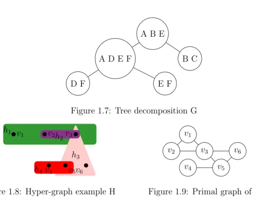
Example 10. Figure 1.8 shows an example of a hyper-graph with X = {v1, v2, v3, v4, v5, v6} and H = {h1, h2, h3, h4} = {{v1, v2, v3},{v2, v3},{v3, v5, v6},{v4}}. The primal graph of H is shown in figure 1.9.
A B E
A D E F B C
D F E F
Figure 1.7: Tree decomposition G v1 v2 v3
v4 v5v6
h1
h2
h3 h4
Figure 1.8: Hyper-graph example H
v1
v2 v3
v4 v5
v6
Figure 1.9: Primal graph of H
Definition 33. (Cut-width and tree-width of a hyper-graph)[44] The cut-width and the tree-width of a hyper-graph are the cut-width and the tree-width respectively of its primal graph plus one.
Definition 34. (Constraint Satisfaction Problem (CSP)) ACSP instance is a triple (V, D, C) where:
• V is an ordered set of n variables (vi is the ith element of v).
• D is a mapping from V to a set of domains {d(v1), d(v2), .., d(vn)}. For each variable vi ∈V , d(vi) is the finite domain of its possible values.
• C ={c1, c2, .., cm} is a set of m constraints. Each constraint ci ∈ C is defined as a pair (vars(ci), rel(ci)), where:
– vars(ci) = (vi1, .., vik)is an ordered subset of V called the constraint scope.
– rel(ci)is a subset of the Cartesian productd(vi1)∗..∗d(vik)and it specifies the allowed combinations of values for the variables in vars(ci).
Definition 35. (Cut-width and tree-width of a constraint satisfaction problem)[44]
The cut-width and the tree-width of a constraint satisfaction problem are the cut- width and the tree-width respectively of its constraint hyper-graph.
Theorem 9. [44] Given a constraint satisfaction problemP and a tree decomposition D of P, P can be solved in O(|P|tw(D)+1·log|P|).
Definition 36. (Cut-width and tree-width of a Petri net) The cut-width and the tree-width of a Petri-net N = (P, T, w) are the cut-width and the tree- width respectively of its underlying hyper-graph HN = (P, H) with H = {{p∈P |w(p, t)6= 0 or w(t, p)6= 0} |t∈T}.
Definition 37. Given a Petri net N = (P, T, w) such that P = {p0, . . . , pn−1}, n ≥2, the constraint satisfaction problem CSP(N) = (V,D,C) for finding a siphon of a parametric size K in N has the following constraints C on the variables V = {X0, S0, . . . , Xn−1, Sn−1, K}.
• for all 0≤i < n, Xi = 1⇒V
t∈•pi
W
pj∈•tXj = 1,
• S0 =X0+X1 and for 1≤i < n−1, Si =Si−1+Xi+1,
• Sn−1 =K
Given a Petri netN, definition 37 provides an encoding of the problem of finding a siphon of size K in such a manner that we are able to bound the cut-width of CSP(N) by the cut-width of N, we decompose the constraint
n−1
X
i=0
Xi = K into n binaries constraints as illustrated in Example 11.
Example 11. Consider Petri net N depicted in Figure 1.10. The corresponding hyper and primal graphs are shown respectively in Figure 1.11 and Figure 1.12.
S P
E
ES t1
t−1
t2
Figure 1.10: Petri net depicting the enzymatic reaction
E S ES
P h1
h2
Figure 1.11: Hyper-graph of the Petri net depicted in Figure 1.10
E
S ES P
Figure 1.12: Primal graph of the Petri net depicted in Figure 1.10
Boolean variables X0, X1, X2 and X3 are associated respectively to E, S, ES and P. The following CSP= (V,D,C) encodes the problem of finding a siphon of N of size K:
V ={X0, S0, X1, S1, X2, S2, X3, S3, K}
The siphon constraints are:
X0 = 1 ⇒X2 = 1 X1 = 1 ⇒X2 = 1 X2 = 1 ⇒X0 = 1∨X1 = 1
X3 = 1 ⇒X2 = 1 Binary constraints encoding the sum are:
S0 =X0+X1
S1 =S0+X2
S2 =S1+X3 S3 =K
Lemma 2. For all Petri net N, c(CSP(N))≤c(N) + 2.
Proof. Suppose that P = {p0, . . . , pn−1} is enumerated such that LN : pi 7→ i is a numbering of the primal graph of the underlying hyper-graph of N with c(LN) = c(N). Then the numbering LCSP(N) such that for all 0≤i < n, LCSP(N)(Xi) = 2·i, LCSP(N)(Si) = 2·i+1andLCSP(N)(K) = 2·nis such that c(LCSP(N)) = c(N)+2.
Example 12. Consider again the Petri netN of Figure 1.10 and the numbering LN
corresponding to the ordering (E, S, ES, P),we have cLN(N) = 3. The primal graph P corresponding toCSP(N)as defined in 37 is depicted in Figure1.13. OnP, consid- ering the numberingLCSP(N)(Xi) = 2·i, LCSP(N)(Si) = 3·i+1andLCSP(N)(K) = 2·n.
This numbering corresponds the the ordering (X0, S0, X1, S1, X2, S2, X3, S3, K). We have c(LCSP(N))(P) = 5 .
X0
X1
X2 X3
S0
S1 S2
S3 K
Figure 1.13: Primal graph of CSP(N)
Theorem 10. Given a Petri-net N with n places with a numbering LN and an integer K, there exists an algorithm to find a siphon of size K if such a siphon exists in N in O(|N|c(LN)+3·log|N|).
Proof. By lemma 2, c(CSP(LN)) =c(LN) + 2Therefore, tw(CSP(LN))≤c(LN) + 2 by lemma 8. Moreover, |N|=O(|P|). Theorem 9 concludes.
Theorem 11. Given a Petri netN withn places with a numberingLN, and a subset of places Q, there exists an algorithm to find a minimal siphon containing Q in N in O(|N|c(LN)+5·(log|N|)2).
Proof. The constraint satisfaction problem CSP′ obtained from CSP(N)by adding the constraintsXi = 1for allpi ∈Qhas the same cut-width as CSP(N). Therefore, a siphon S containing Q with minimal cardinality can be found by iterating the resolution of CSP′ by a dichotomic search among the values of K between 1 and n. If S is minimal (which can be checked polynomially in O(|N|2)), then this is a minimal siphon containing Q in N. If S is not minimal, then there is no minimal siphon containing Q inN.
Proposition 9. The count of minimal siphons in Petri nets is not polynomially bounded by cut-width.
Proof. Given an integern ≥2, consider the Petri-net N depicted below, which has 2n minimal siphons.
A0 A1 A2 An−1
T0 T1 . . . Tn−1
B0 B1 B2 Bn−1
The cut-width of N is 5. Indeed, the primal graph of the underlying hyper-graph of N is G= (V, E) such that V = {Ai, Bi : 0≤i < n} and E =S
0≤i<n{Ai, Bi} × {Ai+1modn, Bi+1modn}. Gis the non-oriented underlying graph. We have c(G)≤6.
Indeed, the numberingLGsuch that for all0≤i < n,LG(Ai) = 2·i,LG(Bi) = 2·i+1 is such that c(LG) = 4.
1.3.2 Linear Time Complexity Result
We show that, given a parameter k > 0, Rec-MESP can be decided in linear time for Petri nets with tree-width bounded by k. We prove also that given a parameter k >0, deciding the Siphon Trap Property can be done in linear time for Petri nets with tree-width bounded byk. These results follow from Courcelle’s theorem which states that every graph property definable in monadic second-order logic can be decided in linear time on graphs of bounded tree-width. The monadic second-order logic is the extension of the first-order logic that allows quantification over monadic unary predicates (i.e.: sets). Thus, non-unary predicates, as well as functions, may
appear in monadic second-order languages, but they may not be quantified over.
Hence, monadic Second Order logics formulas are built up from atomic formulas using the usual boolean connectives (∨;∧;¬;→;↔), quantification over individual variables and quantification over set variables. It is shown that monadic second- order logic, where quantifications over sets of vertices and sets of edges are used, is a reasonably powerful logical language for which one can obtain decidability results.
Our main theorem states the linear time complexity of the Rec-MESP in Petri nets with bounded tree-width.
Theorem 12. For k > 0, there exists an algorithm to find a minimal siphon con- taining a subset of places Q in linear time for Petri nets of tree-width bounded by k.
Proof. Our theorems are corollaries of the Courcelle’s theorem that declares the following:
Theorem 13. (Courcelle’s theorem)[24] If a class C of graphs is definable in monadic second-order logic (MSO) then for any fixed k > 0, given a k-width tree decomposition of a graph G, there exists a linear-time algorithm which recognizes if G∈C.
Given a Petri-net withnplaces andmtransitions, the incidence between vertices (places and transitions) and edges is represented by a binary relation edge. To separate places from transitions, we introduce the unary predicate place. A siphon is a set of places whose predecessors are also successors.
The fact that a set of placesS is a siphon can be written as the following logical expression:
siphon(S):∀v(v ∈S ⇒place(v))∧ ∃v(v ∈S)∧
∀t(∃v(v ∈S∧edge(t, v))⇒ ∃v(v ∈S∧edge(v, t))) S is minimal when Min-Siphon(S)holds where:
Min-Siphon(S):siphon(S)∧ ∀S′(siphon(S’)∧
∀v(v ∈S′ ⇒v ∈S)⇒ ∀v(v ∈S ⇒v ∈S′)) S contains the given set of places Q is trivially written as:
∀v(v ∈Q⇒v ∈S)
Hence, the existence of a minimal siphonS containing a given set of places Qis represented by the following monadic second order logic expression:
Min-Siphon-containing(Q):∃S(siphon(S)∧ ∀S′(siphon(S’)∧
∀v(v ∈S′ ⇒v ∈S)⇒ ∀v(v ∈S⇒v ∈S′))∧ ∀v(v ∈Q⇒v ∈S))
Theorem 14. For k >