In this paper we study approximate and exact controllability of the linear difference equation x(t) =∑Nj=1Ajx(t−Λj) +Bu(t) inL2, with x(t)∈Cd and u(t)∈Cm , by using as a basic tool a representation formula for its solution in terms of the initial condition, the control and some suitable matrix coefficients. In the case of two-dimensional systems with two delays, we obtain an explicit characterization of approximate and exact controllability with respect to the parameters of the problem. To give an explicit representation of the solutions in (1.1), we first give a recursive definition of the matrix coefficients Ξn that appear in such a representation.
We now define the main concepts that we consider in this paper, namely the approximate and exact controllability of the condition xt = x(t+·)|[−Λmax,0) of (1.1) in the function spaceL2((−Λmax,0) , Cd). Equation (2.4) allows one to immediately obtain the following classical characterization of approximate and exact controllability in terms of the operatorE(T) (cf. [6, Lemma 2.46]). a) System(1.1) is approximately controllable in time T if and only ifRanE(T) is dense in X. b) System(1.1) is exactly controllable in time T if and only if E(T) is surjective. We recall in the following theorem the classical characterizations of approximate and exact controllability in terms of the additional operator E(T)∗, whose proofs can be found, e.g. in [6, Section 2.3.2]. a) System(1.1) is approximately controllable in time T if and only if E(T)∗ is injective, i.e. for every x∈X,.
This term consists of the coefficient of the matrix corresponding to the line σn multiplied by evaluated at the coordinates ξ of the intersection point. Thanks to Proposition 2.7, another possible approach to the controllability of (1.1), which will be extended to the case of incomparable delays in Section 4, is to consider the range of the operatorE(T). We now turn to characterizing the controllability of (1.1) using the operatorE(T) from (2.3) instead of the system augmented by Lemma3.1.
We now give a controllability criterion for (1.1) with respect to the rank of C. Then the following propositions are equivalent. a) System(1.1) is approximately controllable in time T ; (b) System(1.1) is exactly controllable in time T.

Reduction to normal forms
It is clear that if both (A1,B) and (A2,B) are checkable, in general only one of the two matrices A1 and A2 can be put into such a normal form.
Proof of Theorem 4.1(a) and (b)
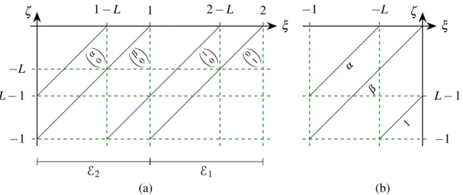
Furthermore, a straightforward calculation has α =a11 and β =a12 on the normal form given in (4.9). RanB), which is not close to inX. IfT <1+L, then the first component of E(T) vanishes for every u∈YT in the non-empty interval(−1,L−T), and therefore the domain of E(T) is not dense inX, which shows that the system is neither approximately nor exactly controllable in timeT<1+L. Therefore, the range of E(T) is not dense in X, showing that the system is neither approximately nor exactly controllable in time T ≥1+Leither.
If T <2, then the first component of E(T)u vanishes for every u∈YT in the non-empty interval (−1,1−T), and therefore the domain of E(T) is not dense in X, which shows that the system is neither approximately nor exactly controllable in time T <2.
Proof of Theorem 4.1(c)
Forn∈N, setn= fn(−1)and let K=min{n∈N|fn T)}. Kis clearly well-defined: ifLis rational, all paths of f are periodic, and therefore K+1 is upper bounded by the period of the cycle starting at −1, and, ifLis irrational, all paths of f are dense in [−1,0 )and therefore they intersect[−1,1−T) infinitely many times.
- Proof of Theorem 4.1(c)(i)
- Proof of Theorem 4.1(c)(ii)
Then the following propositions hold. a) System (4.1) is approximately controllable in some time T ≥2Λ1if and only if it is approximately controllable in time T =2Λ1. To prove the opposite, assume that the system is approximately controllable in time T ≥2 and take x∈X such that E(2)∗x=0 inY2. Then the following propositions hold. a) System(4.1) is approximately controllable for some time T ≥2Λ1if and only if S∗ is injective.
Combining Lemma 4.7 and Theorem 2.8, one obtains that (4.1) in a given time T ≥2 is approximately controllable if and only if E(2)∗ is injective. Combining Lemma 4.7 and Theorem 2.7, one obtains that (4.1) in a given time T ≥2 is exactly checkable if and only if E(2) is surjective. Since M is injective if and only if detM6=0, one concludes that S∗ is injective if and only if 0∈/S, as required.
Since it has already been proved that exact controllability does not hold for T < 2, it suffices to show that, for T ≥2, the system is precisely controllable if and only if 0∈/S. Lemma 4.9 leaves us to show that 0∈/ S if and only if the operator S defined in (4.19) is surjective or, equivalently, if c>0 exists such that S∗ satisfies S∗xkZ ≥ckxkZ for every x∈Z. We say that (1.1) is approximately controllable to constants in time T if RanE(T)⊃K, i.e. for every ∈K and ε>0, there exists u∈YT such that the solutionx of (1.1) with initial condition 0 and controlusatisfieskxT −ykX<ε.
We say that (1.1) is exactly controllable with respect to constants at time T if RanE(T)⊃K, i.e., for each y∈K, there exists su∈YT such that the solutionx of (1.1) with the initial condition 0 and the control satisfy xT =y . As we proved in Lemma2.11 for approximate and exact controllability, approximate and exact controllability over constants is also preserved under linear coordinate change, linear feedback, and time scale changes. a) (1.1) is approximately controllable to constants at time T if and only if (2.8) is approximately controllable to constants at time Tλ;. System (1.1) is exactly controllable to constants at time T if and only if there exists c>0 such that, for each x∈X,.
Then it is clear that Ranκ =K, where K is defined by (5.1), and thus (1.1) is exactly controllable to constants at time T if and only if Ranκ ⊂RanE(T). The main result of this section, Theorem 5.6, states that approximate tractability and approximate tractability on constants are equivalent. As a consequence of Lemma 5.4, we obtain that approximate controllability on constants implies approximate controllability on polynomials.
The result holds for polynomials of degree at most 0, since this is precisely the definition of approximate tractability to constants. Then (1.1) is approximately controllable at time T if and only if it is approximately controllable up to constants at time T.
Exact controllability to constants
Assume that r∈Ni such that for every polynomial p:(−Λmax,0)→Cdof degree at most r and ε >0 there exists u∈YT such that kE(T)u−pkX <ε. We start with the proof that the analog of Lemma 4.7 also holds for exact controllability on constants. Then (4.1) is exactly controllable to constants at some time T ≥2Λ1 if and only if it is exactly controllable to constants at time T =2Λ1.
To prove an analogue of Lemma4.9 for exact controllability to constants, we first introduce the spaceKr(L) defined forL∈(0,1)by. Then (4.1) is exactly controllable to constants in a certain time T ≥2Λ1 if and only if RanS⊃Kr(L), or, equivalently, if there exists c>0, such that, for each x∈Z,. Then Ranκr =Kr(L), which means that (4.1) is exactly controllable to constants in time T ≥ 2 if and only if Ranκr ⊂ RanS.
According to classical results in functional analysis (see e.g. [6, Lemma 2.48]) the last condition is equivalent to the existence of c>0 such that, for any x∈x, . 5.9) You get that by a simple calculation. Then (4.1) is exactly controllable in time T if and only if it is exactly controllable on constants in time T. Note that exact controllability in timeT implies exact controllability on constants in timeT, which in turn implies approximate controllability on constants in timeT, the The latter, thanks to Theorem 5.6, corresponds to an approximate controllability in timeT.
Therefore, the equivalence between exact controllability to constants at time T and exact controllability at time T is especially true when the approximate and exact controllability at time T are equivalent. Therefore, Theorem 5.9 is proved in such situations, and it is left to consider the case when T ≥2Λ1,(A1,B)and(A2,B) are controllable and 0∈S\S. Thanks to Theorem 4.1 (c), (4.1) is not exactly controllable in time T, and so the proposition is proved if one shows that (4.1) is not exactly controllable with respect to constants in time T.
Therefore, thanks to Lemma5.8, (4.1) is exactly controllable for constants in timeT if and only if there existsc>0 such that for everyx∈Z,. Suppose, to obtain a contradiction, that (4.1) is exactly controllable for constants in timeT, and let c>0 be such that (5.10) holds for every x∈Z. Therefore, there exist two sequences (pn)n∈N and (qn)n∈NinZwith, using the inhomogeneous Diophantine approximation theorem (see e.g. [1, Chapter III, Theorem II A]). 5.12) When one remembers that|β|=|α|1−L, one obtains that for each ∈N the eigenvalueλqn ofSbs satisfies.
This contradiction proves that (4.1) is not exactly controllable to time constants T, as required. a) The characteristic polynomial and the determinant of M are given by P(λ). To show that (A.6) holds for everyz∈Caq that zq6=1, it suffices to show that forz∈Cwith|z|<1 holds, since both the left and right sides of (A.6) are the functions meromorphic with simple poles at the roots ofzq=1.