HAL Id: hal-00738384
https://hal.archives-ouvertes.fr/hal-00738384
Submitted on 4 Oct 2012
HAL is a multi-disciplinary open access archive for the deposit and dissemination of sci- entific research documents, whether they are pub- lished or not. The documents may come from teaching and research institutions in France or abroad, or from public or private research centers.
L’archive ouverte pluridisciplinaire HAL, est destinée au dépôt et à la diffusion de documents scientifiques de niveau recherche, publiés ou non, émanant des établissements d’enseignement et de recherche français ou étrangers, des laboratoires publics ou privés.
simulations: a statistical analysis approach
Philippe Caillou, Javier Gil-Quijano, Xiao Zhou
To cite this version:
Philippe Caillou, Javier Gil-Quijano, Xiao Zhou. Automated observation of multi-agent based simula- tions: a statistical analysis approach. Studia Informatica Universalis, Hermann, 2013. �hal-00738384�
simulations
A statistical analysis approach
P. Caillou*, J. Gil-Quijano**, X. Zhou*
* Laboratoire de Recherche en Informatique Université Paris Sud – INRIA, Orsay 91405, France
firstname.name@lri.fr
**CEA, LIST, Laboratoire Information Modèles et Apprentissage, F-91191 Gif-sur-Yvette, France
firstname.name@cea.fr
Résumé. Multi-agent based simulations (MABS) have been successfully used to model complex systems in different areas. Nevertheless a pitfall of MABS is that their complexity increases with the number of agents and the number of different types of behavior considered in the model. For average and large systems, it is impossible to validate the trajectories of single agents in a simulation. The classical validation approaches, where only global indicators are evaluated, are too simplistic to give enough confidence in the simulation. It is then necessary to introduce intermediate levels of validation. In this paper we propose the use of data clustering and automated characterization of clusters in order to build, describe and follow the evolution of groups of agents in simulations. These tools provides the modeler with an intermediate point of view on the evolution of the model. Those tools are flexible enough to allow the modeler to define the groups level of abstraction (i.e. the distance between the groups level and the agents level) and the underlying hypotheses of groups formation. We give an online application on a simple NetLogo library model (Bank Reserves) and an offline log application on a more complex Economic Market Simulation.
Mots-Clés : Complex systems simulation, multi-agents systems, automated observation, auto- mated characterization, clustering, value-test
Studia Informatica Universalis.
1. Introduction
Multi-agent systems (MAS) are specially well suited to represent complex phenomena from the description of local agent behaviours.
The simulation of complex systems using MAS is a cyclic process : the modeler introduces his/her knowledge into the model, runs simula- tions, discovers bugs, pitfalls or unwanted effects, corrects the model and eventually his/her knowledge, and the cycle restarts. The cycle is over when it is not possible to further improve the model because of technical or knowledge limitations.
Once the agents behaviors are defined, the cyclic modeling process usually focuses on fitting global simulation parameters and/or the ini- tial states of agents in order to reproduce global behaviors observed in the modeled empirical phenomena. The global behaviors are usually reproduced and tested with global variables (for example, in the case of socio-spatial models, variables as populations density and growing rates, or evacuation time and number of death for panic simulations).
Those global variables are evaluated both on simulation and on empi- rical data. The calibration of the simulation is achieved by finding the right set of values (or values intervals) for the agents and global simu- lation parameters which lead to minimize the difference between tra- jectories of global variables in simulation and in empirical data. This optimization-like approach is implemented by several existing frame- works (for example in GAMA [TDV10], see section 2 for an extended presentation of these tools).
Nevertheless, this traditional approach may be too simplistic in order to characterize the dynamics of complex systems. Indeed, in a complex system, different phenomena may simultaneously occur at different le- vels (at the agents and at the global levels, but also at intermediate levels) and influence each other [GQLH10]. For instance, groups of agents (flocks of birds, social groups, coalitions, etc.) following simi- lar trajectories of states may appear, evolve and disappear. To describe and evaluate the evolution of that type of groups, the observation of global variables is not enough. Moreover, because of the emergent pro- perties of complex systems, those groups may be unexpected, and their presence may even be unnoticed because no global variable or any other
adapted observation mechanism is provided in the simulator. The signi- ficance and even the existence of groups may then be hidden by the usually huge amount of information generated in a MAS simulations.
In this paper, we introduce the use of statistical-based tools to assist the modeler in the discovering, following the evolution and describing groups of agents. After an overview of the state of the art (section 2, in section 3, we present two complementary tools, data clustering used to discover and build groups and value test used to automatically describe those groups. In section 4, we present an observation model that uses those tools in order to produce automated analysis of the evolution of groups in MAS simulations illustrated on a NetLogo simple model. We present a more complex offline application in section 5 and conclude in section 6.
2. State of the art
Multi-agent based simulations have been used with a large num- ber of economic, geographic or social applications. There are several available development frameworks for simulation, some of them user- friendly with specific coding language, such as NetLogo [LM], and with the possibility to interface with Java code parts (like GAMA [TDV10]).
Others use only generic language (usually java or C#), such as MO- DULECO [Pha] or Repast [NCV06, RLJ06]. However, none of these platforms integrate any module for automatic group analysis. Based on these platforms, some analyzer tools, such as LEIA [GKMP08], SimEx- plorer [LR] and [Cai10] were developed to generate and analyze auto- matically simulations.
LEIA [GKMP08] is a parameter space browser for the IODA simu- lation framework[KMP08]. It allows the user to instantly make a visual comparison of numerous simulations by seeing all their results in paral- lel. It provides the user with a set of transformation and generation tools for model, and a set of tests to browse the simulations space. Scoring rules are applied to help the user in identifying interesting configura- tions (such as cyclic or regular behaviors).
SimExplorer/OpenMole [LR] is a software, which aims at providing a generic environment for programming and executing experimental de- signs on complex models. The goals are multiple : (1) to externalize the development of the model exploration, in order to make available some generic methods and tools which can be applied in most of the cases for any model to explore ; (2) to favor the reuse of available components, and therefore lower the investment for good quality model exploration applications ; (3) to facilitate a quality insurance approach for model exploration.
[Cai10] is a tool to automatically generate and run new simulations until the results obtained are statistically valid using a chi-square test.
It can generate new simulations and perform statistical tests on the re- sults, with an accuracy that increases gradually as the results are produ- ced. This tool can be applied to any RePast-based simulation. It deduces variables and parameters used and asks the user to choose the configura- tion of interest. New simulations are generated, computed and analyzed until all the independence tests between parameters/variables are valid.
Finally, the test results and their margins of error are presented to the users.
The aim of these tools is to study several simulations (the parame- ter space), to compare their result and analyze them. However, none of them aim at studying one complex simulation to describe it. To explore one simulation, the only existing tools are the integrated tools (such as the NetLogo graphs and logs), which are limited to global or user- defined clusters, and classic data mining on logs. We aim to combine the advantage of online and agent-oriented analysis of NetLogo with the flexibility and descriptive potential of Data Mining tools. Some work using data mining tool to identify groups and describe them had been realised with specific applications, for exemple in the SimBogota simu- lation ([GQPD07][EHT07]). In these simulations, social groups in Bo- gota city regions where identified by data mining, and the group results were perceived by the agent. The goal was however more a multi-scale simulation than a description of simulation dynamic.
3. Analysis tools
In this section, we present the two main tools that we use to auto- matically analyze MAS simulations. To discover the groups of agents we propose to use data clustering, and then value-test evaluations to des- cribe them. These tools are associated in our analysis model (see section 4) in order to automatically describe the evolution of groups and help the modeler to understand what happens in complex simulations.
3.1. Finding the groups : clustering
The goal of clustering algorithms is to "find the structure" of a da- taset. Most of the time, data represent objects or individuals that are described by a given number of variables or characteristics [LPM06].
The dataset’s structure is represented as a partition or a hierarchy of partitions. Every single object is assigned to a given group (cluster) in the partition, or to a several groups (clusters) when considering a hierar- chy of partitions. An object is assigned to a given groupg if it is more similar (the sense of similar varies with the algorithm) to the objects in g than to objects in other groups. The main hypothesis when clustering a dataset is that the structure exists and the goal is to make it evident. Si- milarity between objects usually depends on the distance between them (actually between the vector of variables representing them). One of the most used distance (for quantitative variables) is the Euclidean distance.
As the state of an agent is a vector that includes the instantaneous values of the set of variables that describes the agent’s behavior, we can consider the set of states of all the agents in a simulation as a dataset and then to cluster it. In that way, groups of agents whose states simi- larity is maximal can get formed. To conduct the clustering, the "right"
algorithm and distance measure have to be chosen. Indeed, different clustering algorithms can lead to different results as their underlying hy- pothesis and functionning diverge. In our work, it is the responsibility of the modeler to choose those parameters. By including in our model the Weka machine learning library1, we provide the modeler with a wide list of clustering algorithms and distances functions. In our experiments
1. http ://weka.wikispaces.com/
we used the X-Means algorithm [PM00], described in the following pa- ragraphs.
One of the most known algorithm of clustering is the K-Means algo- rithm [Llo82] whose objective is to find thekprototypes (average cha- racteristic vectors) that represents the best the data. In that algorithmk initial prototypes are defined (usually by random) and at each iteration every object is assigned to its nearest prototype. Every prototype is then updated to the average vector of the characteristics of the objects that were assigned to it. The process is repeated until there is no significant changes of prototypes between two succesive iterations or until a maxi- mum number of iterations is reached. The main pitfall of K-Means is that the numberkof clusters must be known. As the idea of clustering is to find the right and unknown structure describing the dataset, there is no reason to knowkbeforehand.
An improvement of K-Means is proposed with the X-Means algo- rithm [PM00]. In that algorithm the "right" numberk of clusters is de- termined by successive K-Means executions. The first execution starts with akmin number of clusters (the minimum number of clusters, a pa- rameter of the model), and at each iteration one of the clusters found in the previous iterations is divided into two new clusters. The cluster to be divided is the one whose internal similarity (the similarity between the objects inside the cluster) is the lowest. The process is repeated until kmaxnumber of clusters is reached. Thenkmax−kmin+ 1partitions are produced. The chosen partition is the one that maximizes the internal similarity of clusters and maximizes the distance between prototypes.
3.2. Interpreting the groups : Value tests
Value test (VT) [Mor84, LPM06] is an indicator that allows the au- tomated interpretation of clusters. It determines the more significant factors (for continuous variables) and modalities (for categorical va- riables) in a given cluster in comparison with the global dataset. The VT compares the deviation between the variables/modalities in clusters and the variables/modalities in the overall dataset. The main hypothe- sis in the VT calculation is that the variables follow Gaussian distri- butions. In that condition, for a level of risk of 5% we can consider
Figure 1 – Overview of the analysis model
that a variable/modality is significant if its VT is greater than 2. The automated description of a group is given by its set of significant va- riables/modalities. For continous variables the mean value of the va- riable in the group completes the description.
We present here the calculation of V T for continuous variables, for categorical variables see [Mor84]. Given a dataset containing n ele- ments and a cluster k on the dataset containing nk elements. Given a quantitative variablej, its averageE(nj)and its varianceS2(nj)in the overall dataset. Given also the averageE(njk) ofj in the cluster k, the V T for the variablej in the clusterkis computed as follows :
V T(njk) = (E(njk)−E(nj)) p(n−nn−1k × S2n(nj)
k ) (1)
4. Analysis model 4.1. Model overview
Our goal is to describe, online or offline, what happens in a simula- tion at the cluster level. Our model can be described with several steps as illustrated in Fig. 1 :
1) Model Selection : what do we study ? 2) Data processing : what are the data ?
3) Clustering : can we find homogeneous groups ? 4) Cluster description : how can we describe them ? 5) Cluster evolution : how do they evolve ?
6) Simulation generation : is this reproducible ? In future work, we intend to use the most interesting (or user-selected) agent model (clus- ters) identified to generate new simulations with similar agents and thus test the clusters behavioral stability.
For a better understanding, we will describe each step with the ap- plication of our tool to an illustrative example.
4.2. Model selection
The first step is to choose the model to be studied. Our model can be applied both online (with NetLogo) or offline from logs (by simulating an online data stream).
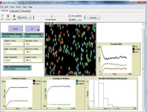
We choose here the Bank Reserves model, provided with Netlogo, where financial agents either save or borrow money via loans (Fig. 2).
This is a very simple model illustrating the effect of money creation via savings deposits/loans grants. There is only one Bank andP eople (consumers) agents. Each agent begins with a random amount of money in its wallet (between 0 and a parameter richT hreshold). When an agent has a positive wallet, it deposits its money in the bank, which increases itssavingvariable (and puts itswalletat 0).
At each step, agents move randomly. When they meet someone they make a transaction, which is a simple transfer from one agent to the
Figure 2 – Netlogo Bank Reserves Model
other. When the buyer agent has not enough money (savingsorwallet), he takes aloan. The bank grants loans (and creates money) unless the total amount of loans reaches the total amount of deposits (savings) multiplied by a parameter (1-Reserves). In other words, the bank has to keep a Reserve proportion of its deposits which can not be used for loans. When an agent receives money (via transactions), it uses it to pay back its loans if it has some. Thewealth of an agent is defined as savings+wallet−loans. For our illustrative experiment, we use Reserves= 70,P eople= 200andrichT hreshold= 20.
NetLogo provides some tools to observe an experiment either at an individual or at a global level. For example, on Fig.2 some global va- riables are presented to give an overview of an experiment. The global amount ofloans and money show an early increase, then a stabiliza- tion of the totalmoneywhen the maximum amount ofloansis reached.
The Income distribution graph gives an overview of the repartition of wealth between three fixed groups (negative wealth, wealth higher
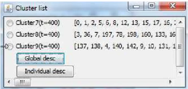
Figure 3 – The cluster list panel gives the identity number of the agents included in each cluster.
thanrichT hresholdand the rest). Even if these informations are inter- esting, a more detailed understanding of the model behavior can not be reached with such global/local observation. For example, it is difficult to answer the following questions : who are the wealthy agents ? Do the rich stay rich ? This would even be truer for more complex models, for which variable interactions are much more difficult to deduce than with such a simple toy simulation.
4.3. Data processing
A data matrix is generated every n steps. A line in the matrix re- presents one agent’s state. Raw data from simulations are not the only interesting data for cluster’s generation and analysis. Several filters or aggregators can also be used to process the data stream. We use two different aggregators to complete the initial matrix : i) the moving ave- rage (for each variable, we add a new variable computed as the average of the last five steps values) ; ii) the initial values for each agent (for each variable, we define a new variable corresponding to the value of the variable for this agent at the starting point of the simulation). These initial values variables are not used in the clustering but used latter for the description of the clusters.
4.4. Clustering
Clustering is performed on the final data in order to generate homo- geneous agent groups (for now, X-Means is used, but any other cluste- ring algorithm from Weka can be easily selected instead). Clusters are visualized in NetLogo (with colors), and their extension and descrip- tion are presented. For example, in Fig. 3, three clusters are identified in t=400.
4.5. Cluster’s description
Once the clusters are identified, it is possible to get an easy-to-read description by usingV T (see sec. 3.2). The description withV T (Fig.
4) makes it easy to interpret and describe them. Positively (respectively negatively) significant variables are presented in blue (resp. red) : their average is significantly higher (resp. lower) than the global average.
For example, int = 400, three clusters are identified.Cluster7, with 114 agents, is a "poor" cluster, whose agents have lowwealth,savings, walletand the corresponding moving average variables (M M savings andM M wealth), and a higher amount of loans. Some significant va- riables are (probably) clustering artifacts (Y Cor) or random effects (T OHeading), and will justify our stability analysis.
Similarly, cluster9 regroups the 66 ”wealthy” people, with high wealthandsavingsand fewloans. An interesting result is the signifi- cantT0W alletvariable, corresponding to thewalletvalue of agents at the beginning of the simulation. Thewealthypeople were significantly richer than the average at the beginning of the simulation.
At the end of the simulation, a description of all the clusters obtained at each time step gives a global overview of the simulation (Fig. 5, with a selection of some results in Table 1). In our experiment, it is always possible to identify awealthyand apoorcluster, and sometimes (like in t = 400) amiddlecluster. From their description, it is already possible to observe that the link between the wealthand the initial wealth (the T0W allet) is not significant anymore aftert = 400. It may be related to the fact (observed with NetLogo global observation) that bank has
Figure 4 – Cluster Description at t=400 : listed variables are higher for the member of the cluster (blue positive value) of lower (red negative values) than in the global population. Black variables are not signifi- cantly different.
Figure 5 – Global Overview of clusters
reached its loan limit (the total amount of money stops to increase at aroundt = 230).
However, it is difficult to compare clusters at different time steps with this overview since they are different both in intension and in extension.
In a more complex model, cluster may have a completely different mea- ning at different steps.
Tableau 1 – Selection of the “rich” clusters and some variables results from the global overview of a simulation (Fig 5)
VT Cluster6 Cluster9 Cluster10 Cluster13
time 200 400 600 800
size 95 66 37 52
Savings 11,25 9,68 11,29 3,26
Loans -6,5 -3,93 -2,63 -1,77
Wealth 10,87 8,91 9,72 3,27
TOWallet 3,16 2,81 0,46 -0,11
4.6. Clusters evolution
In order to describe the clusters’ evolution, we consider two alterna- tive hypothesis : either the extension in every cluster is considered as stable (we keep exactly the same agent population in the cluster), or the intension of every cluster is fixed (we keep the same definition of the cluster).
Evolution by extension/population
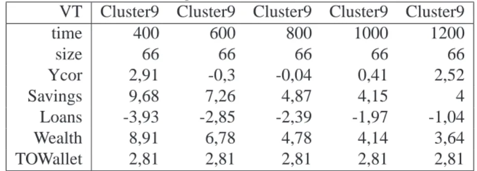
Once an interesting cluster is identified (for example the wealthy agents oft= 400, cluster9), it is interesting to follow its evolution. To do it, the first way is to fix the extension (population) of the cluster.
Fig.6 describes the evolution of the cluster9 with fixed extension after t = 400 (see Table 2 for a selection of the most interesting va- riables). Initial parameters values are stable since the population does not change. Other variables may change (except for example Idsince this variable is constant for every agent). This view clearly shows that all wealth-related differences with the other agents decrease : all the (ab-
Figure 6 – Cluster evolution of Cluster9 (rich peoples of T=400) by extension (fixed population)
solute)V T values forwealth, saving andloans decrease. This mean that, in average, the wealthy people of t = 400are becoming less and less wealthy. They are still significantly wealthier than the average at t= 1200, but theirloansare no more significantly lower in comparison witht = 1000. We can also check on this evolution that the clustering artifacts (like theY Corvariable) do not stay significant.
Evolution by definition
The second way is to fix the clusters intension (definition). Fig. 7 represents the description of the clusters identified at each step with the intension function oft = 400(see Table 3 for a selection of interesting variables). All the variables considered in clustering are by definition roughly similar, since the intension of clusters is the same. However, the other variables may evolve (in our example, the initial parameters of the agents).
Tableau 2 – Evolution of Cluster9 (rich peoples of T=400) by extension : selection of some interesting variables
VT Cluster9 Cluster9 Cluster9 Cluster9 Cluster9
time 400 600 800 1000 1200
size 66 66 66 66 66
Ycor 2,91 -0,3 -0,04 0,41 2,52
Savings 9,68 7,26 4,87 4,15 4
Loans -3,93 -2,85 -2,39 -1,97 -1,04
Wealth 8,91 6,78 4,78 4,14 3,64
TOWallet 2,81 2,81 2,81 2,81 2,81
Cluster9, for example, regroup the wealthy agents at each step, but the number and the initial properties of these agents evolve. It is inter- esting to see that the number of wealthy agent stays approximatively constant (66, 71, 56, 58, 65). But the evolution of the initial parame- ters confirms the observation made with the global overview : the ini- tial wealth of the agent (T OW allet) is not significant anymore after t= 600.
Tableau 3 – Evolution of Cluster9 (rich peoples defined at T=400) by definition : selection of some interesting variables
VT Cluster6 Cluster6 Cluster6 Cluster6
time 400 600 800 1000
size 66 71 56 58
Savings 9,68 9,38 9,04 8,61
Wealth 8,91 8,96 8,52 8,49
T0Heading 2,52 1,84 1,47 1,24
T0Wallet 2,81 2,23 0,91 1,48
4.7. Cluster evaluation
The evaluation of the cluster is done by combining the size of the cluster and its ‘descriptivness’ measured by the number of significant V T. The objective is to identify clusters that are both big enough to be generic and descriptive enough to bring some interesting informations.
Figure 7 – Cluster evolution of Cluster9 (rich peoples defined at T=400) by intension (fixed definition)
The score of a cluster c at time step t is calculated as the product of the number of significant variables (whose ‘|V T| is greater than 2) : score(c, t) = |Vc,tS| ×nc,twhereVc,tS is the set of significant variables of candnc,tis the number of agents incat the timet.
For example, in Fig. 6, the score of the cluster is initially relatively high (924) because the population is important and the number of si- gnificantV T is high. But since the cluster is not stable (the rich people don’t stay rich), the number of significant variables decreases. The score decreases, reflecting the fact that the cluster becomes difficult to inter- pret (except by : "the ones that were poor at t=400").
5. Experiments
We tested our analysis tool on several simulation models, both on- line with NetLogo and offline with data logs. Since we have already described a NetLogo application in the previous section to illustrate the description tool, we will describe here an offline analysis application.
Model description
To illustrate how our model deals with more complex simulations, we chose a model following the KIDS approach [EM04] : the number of parameters and observed variables is kept high to be more descrip- tive and realistic rather than synthetic. The Rungis Wholesale Market simulation [CCB09a][CCB09b] was developed with the BitBang Fran- mework [BMC06] and reproduces a Fruit and Vegetable wholesale mar- ket. One type of seller agent and 4 types of Buyer agents are conside- red in the simulation (with many variable parameters, 20 variables in average by agent type). The four type of buyer agents are : Restora- tors seeking efficiency, TimeFree seeking good opportunities, Barbes seeking low-quality and low price products and Neuilly buyers seeking high quality high prices products. The csv logs record one line for each couple day/agent, with 33 output variables (see below). We analyze here only the 60 Buyer agents during the first 10 days of the simulation.
The main observed variables of this model are the transaction time, the number of sellers per buyer, the quality and quantity of the products and the prices. There are four types of prices, the producer price (price
paid by the sellers to the producers), the transaction price(price paid by the buyers to the sellers), the standard price (price given at the beginning of the transaction) and the final price (price paid by the consumers).
In general producerprice < transactionprice < standardprice <
f inalprice.
Clusters description
Two clusters are identified at each step. They are easy to describe since many variables are significant (see Fig 8 where the high propor- tion of red or blue numbers illustrates the high number of significant variables, and a selection and description of interesting variables for the cluster 3 in Table 4). For example, at t=0 (and t=1) we identify the “ex- pansive” cluster that is composed by the buyers of high-quality expan- sive products, and the “cheaps” cluster that is composed by the agents buying low-quality cheap products. Even if this could be anticipated from the buyers definition, one first quick analysis helps to validate the model behaviors : the “expansive” products are fresher (product Age), with higher prices, and the Buyer and Seller profit as well as profit rate higher than for the “cheaps”. Other significant variables give some new interesting informations : the buying time (M oyHour) is not si- gnificantly different, but the expansive buy significantly more products (Sumof Qty) to more Sellers (N bSeller) than the cheaps agents. These informations were not trivial to identify unless you knew you want to find it before the analysis.
Cluster’s evolution
Following the identified clusters brings new interesting insights. For example, in Fig. 9 (and some selected variables in Table 5), we fol- low the “expansive” cluster identified at t=1. First, it is possible to check that the clusters has a stable behavior. The agents buying expan- sive and high-quality products still do the same in the following days.
It is however possible to describe some cluster evolutions : the Moy- Hour variable, which measures the Average transaction time shows a constant decrease. “expansive” agents buy progressively sooner than the “cheaps” agents. Also, the SumQty variables, which was signifi- cant when the cluster was created, becomes quickly not-significant : the
Figure 8 – Global Overview of clusters after 10 days of Rungis Market Simulation
Tableau 4 – Variable selection and description for the cluster3 identified at t=1
Cluster Variable description 4
Pop Cluster size 25
MoyHour Avg Time for transaction -1,76 NbSeller Nb of visited sellers 2,26
SumQty Total Bought Qty 2,43
NbProd Nb of product category 2,26 MoyTransPrice Avg Transaction Price 5,89 MoyFinPrice Avg Price for final consummer 6,1 MoyStdPrice Avg Starting Price 5,72 MoyProdPrice Avg Producer Price 3,09 MoyAge Avg Age of the product -5,59
MoyQuality Avg Quality 6,18
MoyQty Avg Qty for transactions -1,05 MoymargBuyer Avg Buyer margin rate 3,76 MoymargSeller Avg Seller margin rate 5,29
expansivebuyers do not buy more product thant the orthers, it was just an artifact at the cluster creation.
6. Conclusions
The framework for the observation of MAS simulation that we present here, provides the modeller with generic tools that allow him/her to get a synthetic descriptive view of MABS. Presently, it can be used to understand the dynamics of simulations and to ease their validation. In future work we intend to develop a mechanism that will allow the mo- deller to use the definitions of interesting clusters in new simulations as generic “agent models”. Indeed, cluster definition and population can be used to define a distribution function to generate agents profiles.
It is easy to retrieve the average values and the standard deviation of every variable by using simple statistical analysis tools. Agents gene- rated using the distribution functions could be reintroduced in simula- tions, clusters can be rebuilt and the global simulation variables can be
Tableau 5 – Evolution by extension of theexpansivegroup detected at t=1 (cluster3)
Day 1 2 3 4 5 6
Pop 25 25 25 25 25 25
MayHour -1,76 -2,22 -3,37 -3,21 -2,85 -3,61 NbSeller 2,26 1,3 0,77 0,63 1,99 -1,12 SumQty 2,43 1,82 0,83 1,3 3,53 -0,53 NbProd 2,26 1,3 0,77 0,63 1,99 -1,12 MoyTransPrice 5,89 4,52 5,14 5,09 5,84 4,42 MoyFinPrice 6,1 5,36 5,38 5,67 6,25 5,5 MoyStdPrice 5,72 3,42 2,87 3,28 4,84 2,8 MoyProdPrice 3,09 0,88 2,32 2,94 3,48 1,96 MoyAge -5,59 -4,73 -4,77 -5,34 -5,57 -4,91 MoyQuality 6,18 4,96 5,23 5,59 6,16 5,14 MoyQty -1,05 0,63 -0,13 1,03 1,79 1,33
MoymargBuyer 3,76 5 4,14 4,91 4,76 4,77
MoymargSeller 5,29 3,95 4,45 3,97 4,83 3,95
Figure 9 – Evolution by extension of theexpansive group detected at t=1 (cluster3)
compared with their previous values. In that way, the clusters stability and their "expressiveness" can be measured over different simulations.
In order to allow the analysis of a wide number of different type of simulations we are currently adapting our framework both to consider qualitative and network variables and facilitate large simulations analy- sis. The latter will be done by integrating our framework to the Open- Mole engine. That engine provides, among other facilities, the easy use of cluster and grid computing for simulations.
Références
[BMC06] T. Baptista, T. Menezes, and E. Costa. Bitbang : A model and framework for complexity research. In ECCS 2006, 2006.
[Cai10] Philippe Caillou. Automated multi-agent simulation gene- ration and validation. In PRIMA 2010, page 16p. LNCS, 2010.
[CCB09a] Philippe Caillou, Corentin Curchod, and Tiago Baptista.
Simulation of the rungis wholesale market : Lessons on the calibration, validation and usage of a cognitive agent-based simulation. In IAT, pages 70–73, 2009.
[CCB09b] Corentin Curchod, Philippe Caillou, and Tiago Baptista.
Which Buyer-Supplier Strategies on Uncertain Markets ? A Multi-Agents Simulation. In Strategic Managemtn So- ciety, Washington États-Unis d’Amérique, 2009.
[EHT07] Bruce Edmonds, Cesareo Hernandez, and Klaus Troitzsch, editors. Social Simulation : Technologies, Advances and New Discoveries, volume 1. Idea Group Inc., 2007.
[EM04] Bruce Edmonds and Scott Moss. From kiss to kids - an ’anti-simplistic’ modelling approach. In MABS, pages 130–144, 2004.
[GKMP08] Francois Gaillard, Yoann Kubera, Philippe Mathieu, and Sebastien Picault. A reverse engineering form for multi agent systems. In ESAW 2008, pages 137–153, 2008.
[GQLH10] Javier Gil-Quijano, Thomas Louail, and Guillaume Hutz- ler. From biological to urban cells : lessons from three multilevel agent-based models. In PRACSYS 2010 – First Pacific Rim workshop on Agent-based modeling and simu- lation of Complex Systems, Kolkota, India, 2010. LNCS.
[GQPD07] J. Gil-Quijano, M. Piron, and A. Drogoul. Mechanisms of automated formation and evolution of social-groups : A multi-agent system to model the intra-urban mobilities of Bogotá city. In Social Simulation : Technologies, Ad- vances and New Discoveries, chapter 12, pages 151–168.
Idea Group Inc., 2007.
[KMP08] Yoann Kubera, Philippe Mathieu, and S ?bastien Picault.
Interaction-oriented agent simulations : From theory to im- plementation. In Malik Ghallab, Constantine Spyropoulos, Nikos Fakotakis, and Nikos Avouris, editors, Proceedings of the 18th European Conference on Artificial Intelligence (ECAI’08), pages 383–387. IOS Press, 2008.
[Llo82] Stuart P. Lloyd. Least squares quantization in pcm. In IEEE Transactions on Information Theory, volume 28, pages 129–137, 1982.
[LM] Center For Connected Learning and Computer-Based Mo- deling. Netlogo : http ://ccl.northwestern.edu/netlogo/.
[LPM06] Ludovic Lebart, Marie Piron, and Alain Morineau. Statis- tique exploratoire multidimeensionnelle : visualisation et inférence en fouilles de données. Fourth edition, Dunod, Paris, 2006.
[LR] Mathieu Leclaire and Romain Reuillon. Simexplorer : http ://www.simexplorer.org/.
[Mor84] Alain Morineau. Note sur la caractérisation statistique d’une classe et les valeurs-tests. In Bull. Techn. du Centre de Statistique et d’Informatique Appliquées, volume 2, pages 20–27, 1984.
[NCV06] Michael J. North, Nicholson T. Collier, and Jerry R. Vos.
Experiences creating three implementations of the repast agent modeling toolkit. In ACM Transactions on Modeling and Computer Simulation, volume 16, pages 1–5, 2006.
[Pha] Denis Phan. From agent-based computational economics towards cognitive economics. In Cognitive Economics, Handbook of Computational Economics.
[PM00] Dan Pelleg and Andrew Moore. Xmeans : Extending k- means with efficient estimation of the number of clusters.
In 17th International Conference on Machine Learning, pages 727–734, 2000.
[RLJ06] Steven F. Railsback, Steven L. Lytinen, and Stephen K.
Jackson. Agent-based simulation platforms : Review and development recommendations. In Simulation, volume 82, pages 609–623, 2006.
[TDV10] Patrick Taillandier, Alexis Drogoul, and Duc-An Vo.
Gama : a simulation platform that integrates geographi- cal information data, agent-based modeling and multi-scale control. In PRIMA 2010, 2010.