HAL Id: hal-00342825
https://hal.archives-ouvertes.fr/hal-00342825
Preprint submitted on 1 Dec 2008
HAL is a multi-disciplinary open access archive for the deposit and dissemination of sci- entific research documents, whether they are pub- lished or not. The documents may come from teaching and research institutions in France or
L’archive ouverte pluridisciplinaire HAL, est destinée au dépôt et à la diffusion de documents scientifiques de niveau recherche, publiés ou non, émanant des établissements d’enseignement et de recherche français ou étrangers, des laboratoires
Bayesian calibration of the nitrous oxide emission module of an agro-ecosystem model
Simon Lehuger, Benoit Gabrielle, Marcel van Oijen, David Makowski, Jean-Claude Germon, Thierry Morvan, Catherine Hénault
To cite this version:
Simon Lehuger, Benoit Gabrielle, Marcel van Oijen, David Makowski, Jean-Claude Germon, et al..
Bayesian calibration of the nitrous oxide emission module of an agro-ecosystem model. 2008. �hal- 00342825�
Bayesian calibration of the nitrous oxide emission module of an agro-ecosystem model
S. Lehuger
a 1, B. Gabrielle
a, M. Van Oijen
b, D. Makowski
c, J.-C. Germon
d, T. Morvan
e, C. H´enault
da: Institut National de la Recherche Agronomique, UMR 1091 INRA-AgroParisTech Environnement et Grandes Cultures, 78850
Thiverval-Grignon, France
b: Centre for Ecology and Hydrology-Edinburgh, Bush Estate, Penicuik, UK c: Institut National de la Recherche Agronomique, UMR 211
INRA-AgroParisTech Agronomie, Thiverval-Grignon, France
d: Institut National de la Recherche Agronomique, UMR 1229 Microbiologie du sol et de l’environnement, Dijon, France
e: Institut National de la Recherche Agronomique, UMR 1069
INRA-Agrocampus Sol Agro et hydrosyst`eme Spatialisation, Rennes, France
1Corresponding author: UMR1091 INRA, AgroParisTech Environnement et Grandes Cultures, 78850 Thiverval-Grignon, France. E-mail: Simon.Lehuger@grignon.inra.fr Fax: (+33) 1 30 81 55 63 Phone: (+33) 1 30 81 55 24
Abstract
1
Nitrous oxide (N2O) is the main biogenic greenhouse gas contributing to the global warming
2
potential (GWP) of agro-ecosystems. Evaluating the impact of agriculture on climate there-
3
fore requires a capacity to predict N2O emissions in relation to environmental conditions and
4
crop management. Biophysical models simulating the dynamics of carbon and nitrogen in agro-
5
ecosystems have a unique potential to explore these relationships, but are fraught with high
6
uncertainties in their parameters due to their variations over time and space. Here, we used a
7
Bayesian approach to calibrate the parameters of the N2O submodel of the agro-ecosystem model
8
CERES-EGC. The submodel simulates N2O emissions from the nitrification and denitrification
9
processes, which are modelled as the product of a potential rate with three dimensionless factors
10
related to soil water content, nitrogen content and temperature. These equations involve a total
11
set of 15 parameters, four of which are site-specific and should be measured on site, while the
12
other 11 are considered global, i.e. invariant over time and space. We first gathered prior informa-
13
tion on the model parameters based on literature review, and assigned them uniform probability
14
distributions. A Bayesian method based on the Metropolis-Hastings algorithm was subsequently
15
developed to update the parameter distributions against a database of seven different field-sites
16
in France. Three parallel Markov chains were run to ensure a convergence of the algorithm. This
17
site-specific calibration significantly reduced the spread in parameter distribution, and the un-
18
certainty in the N2O simulations. The model’s root mean square error (RMSE) was also abated
19
by 73% across the field sites compared to the prior parameterization. The Bayesian calibration
20
was subsequently applied simultaneously to all data sets, to obtain better global estimates for
21
the parameters initially deemed universal. This made it possible to reduce the RMSE by 33%
22
on average, compared to the uncalibrated model. These global parameter values may be used
23
to obtain more realistic estimates of N2O emissions from arable soils at regional or continental
24
scales.
1
Keywords
2
Bayesian calibration; Parameter uncertainty; CERES-EGC, Nitrous oxide; Markov Chain Monte
3
Carlo; Greenhouse gases
4
1 Introduction
1
Soils are the main source of nitrous oxide (N2O) in the atmosphere, via the microbial processes of
2
nitrification and denitrification. Because of its heavy reliance on synthetic N-fertilisers, agricul-
3
ture has enhanced these two processes, as a result of which agro-ecosystems contribute 55-65%
4
of the global anthropogenic emissions of N2O. Compared to other ecosystem types or economic
5
sectors, they are thus responsible for the major part of the atmospheric build-up of N2O (Smith
6
et al., 2007). Compared to other greenhouse gases (GHG) such as CO2, N2O fluxes are of small
7
magnitude and highly variable in space and time, being tightly linked to the local climatic se-
8
quence and soil properties. Predicting N2O emissions from agro-ecosystems thus requires taking
9
into account complex processes and interactions which originate from both environmental con-
10
ditions and agricultural practises (Duxbury and Bouldin, 1982; Grant and Pattey, 2003; Pattey
11
et al., 2007). This poses a serious challenge to the estimation of the source strength of arable
12
soils, which is currently mostly based on available statistics on fertilizer ignoring these environ-
13
mental factors (IPCC, 2006; Lokupitiya and Paustian, 2006). On the other hand, process-based
14
agro-ecosystem models may in principle capture these effects, and have thereby a unique poten-
15
tial to predict N2O emissions from arable soils at the plot-scale as well as at regional and con-
16
tinental scales (Butterbach-Bahl et al., 2004; Li et al., 2001; Gabrielle et al., 2006a; Del Grosso
17
et al., 2006). Examples of biophysical N2O-models include DAYCENT (Parton et al., 2001),
18
DNDC (Li, 2000), FASSET (Chatskikh et al., 2005) and CERES-EGC (Gabrielle et al., 2006b).
19
However, a major limitation to the wide-spread use of these models lies in the fact that their
20
predictions are highly dependent on parameter settings, and carry a large uncertainty due to un-
21
certainties in parameter values, driving variables and model structure (Gabrielle et al., 2006a).
22
Although model parameterisation and uncertainty analysis are widely developed in the litera-
23
ture on agro-ecosystem models, they are rarely considered simultaneously (Monod et al., 2006;
24
Makowski et al., 2006). Bayesian calibration makes it possible to combine the two types of anal-
1
ysis by providing estimates of parameters values under the form of probability density functions
2
(pdfs), which may be also propagated to model outputs as pdfs (Gallagher and Doherty, 2007).
3
Probability density functions are initially the expression of current imprecise knowledge about
4
model parameter values, this prior probability is then updated with the measured observations
5
into posterior probability distribution by means of Bayes’ theorem (Makowski et al., 2006).
6
In ecological and environmental sciences, Bayesian calibration has been applied to a wide range
7
of models (Hong et al., 2005; Larssen et al., 2006; Ricciuto et al., 2008), and this field is de-
8
veloping actively, mainly using Markov Chain Monte Carlo (MCMC) methods to estimate the
9
posterior pdf for the model parameters. The Bayesian methodology described by Van Oijen et al.
10
(2005) was applied to dynamic process-based forest models with the objective of calibrating
11
model parameters with various types of observed data from forested experimental sites (Svens-
12
son et al., 2008; Klemedtsson et al., 2007). In these examples, Metropolis-Hastings MCMC-
13
algorithm was used to generate samples from the posterior parameter distributions. Although
14
there is an increasing body of literature on the application of Bayesian approaches to environ-
15
mental sciences, the latter have not been applied to process-based model of soil N2O emission
16
models, to the best of our knowledge.
17
The overall purpose of this paper was thus to calibrate the parameters of the N2O emission mod-
18
ule of the CERES-EGC agro-ecosystem model and to quantify uncertainty of model simulations
19
by developing a suitable Bayesian calibration method. Data sets of measured N2O emission rates
20
were collected from seven field-sites in Northern France, which represent major soil types, crops
21
and management practices of the area. The Bayesian procedure was first applied separately to
22
each experimental site, and secondly to the ensemble of the sites. This made it possible to ex-
23
plore the spatial variability of model parameters, and to test whether they could be considered as
24
universal and with which uncertainty range.
25
2 Material and Methods
1
We carried out Bayesian calibration using the Metropolis-Hastings algorithm, to estimate the
2
joint probability distribution for the parameters of the N2O emission module of the CERES-
3
EGC model. The equations of this module involve 15 parameters, of which 11 were considered
4
as global (i.e. invariant over time and space) by the model’s author, the remaining 4 being site-
5
specific (H´enault et al., 2005). While the latter were laboratory-measured in all experimental
6
sites and set to the resulting values throughout, the subset of 11 global parameters was estimated
7
by our Bayesian procedure. We collated a database of N2O flux measurements including 7
8
different field-sites in France, and various N fertilizer forms and rates in 2 of the sites. Bayesian
9
calibration was applied either to each site or treatment individually, or directly to the ensemble
10
of the data sets.
11
2.1 The CERES-EGC model
12
2.1.1 A process-based agro-ecosystem model
13
CERES-EGC was adapted from the CERES suite of soil-crop models (Jones and Kiniry, 1986),
14
with a focus on the simulation of environmental outputs such as nitrate leaching, emissions of
15
N2O and nitrogen oxides (Gabrielle et al., 2006a). CERES-EGC runs on a daily time step, and
16
requires daily rain, mean air temperature and Penman potential evapo-transpiration as forcing
17
variables. The CERES models are available for a large number of crop species, which share the
18
same soil components (Jones and Kiniry, 1986).
19
CERES-EGC comprises sub-models for the major processes governing the cycles of water, car-
20
bon and nitrogen in soil-crop systems. A physical sub-model simulates the transfer of heat, water
21
and nitrate down the soil profile, as well as soil evaporation, plant water uptake and transpiration
22
in relation to climatic demand. Water infiltrates down the soil profile following a tipping-bucket
23
approach, and may be redistributed upwards after evapo-transpiration has dried some soil layers.
24
In both of these equations, the generalised Darcy’s law has subsequently been introduced in order
1
to better simulate water dynamics in fine-textured soils (Gabrielle et al., 1995).
2
A biological sub-model simulates the growth and phenology of the crops. Crop net photosynthe-
3
sis is a linear function of intercepted radiation according to the Monteith approach, with intercep-
4
tion depending on leaf are index based on Beer’s law of diffusion in turbid media. Photosynthates
5
are partitioned on a daily basis to currently growing organs (roots, leaves, stems, fruits) accord-
6
ing to crop development stage. The latter is driven by the accumulation of growing degree days,
7
as well as cold temperature and day-length for crops sensitive to vernalisation and photoperiod.
8
Lastly, crop N uptake is computed through a supply/demand scheme, with soil supply depending
9
on soil nitrate and ammonium concentrations and root length density.
10
A micro-biological sub-model simulates the turnover of organic matter in the plough layer. De-
11
composition, mineralisation and N-immobilisation are modelled with three pools of organic mat-
12
ter (OM): the labil OM, the microbial biomass and the humads. Kinetic rate constants define the
13
C and N flows between the different pools. Direct field emissions of CO2, N2O, NO and NH3
14
into the atmosphere are simulated with different trace gas modules.
15
2.1.2 The nitrous oxide emission module
16
This module simulates the production of N2O in soils through both the nitrification and the
17
denitrification pathways, and was adapted from the semi-empirical model NOE (H´enault et al.,
18
2005). The denitrification component is derived from the NEMIS model (H´enault and Germon,
19
2000) that calculates the actual denitrification rate (Da, kg N ha−1 d−1) as the product of a
20
potential rate at 20 °C (PDR, kg N ha−1 d−1) with three unitless factors related to water-filled
21
pore space (FW), nitrate content (FN) and temperature (FT) in the topsoil, as follows:
22
Da =P DR FN FW FT (1)
In a similar fashion, the daily nitrification rate (Ni, kg N ha−1 d−1) is modelled as the product
1
of a maximum nitrification rate at 20 °C (MNR, kg N ha−1 d−1) with three unitless factors
2
related to water-filled pore space (NW), ammonium concentration (NN) and temperature (NT)
3
and expressed as follows:
4
N i=M N R NN NW NT (2)
Nitrous oxide emissions resulting from the two processes are soil-specific proportions of total
5
denitrification and nitrification pathways, and are calculated according to:
6
N2O =r Da+c N i (3)
where r is the fraction of denitrified N and c is the fraction of nitrified N that both evolve as N2O.
7
The N2O sub-model of CERES-EGC involves a total set of 15 parameters of which four of them
8
are site-specific and must be measured on site, while the other 11 are considered global, i.e. in-
9
variant over time and space. The local (site-specific) parameters are the potential denitrification
10
rate (PDR), the maximum nitrification rate (MNR) and the fractions of nitrified (c) and denitri-
11
fied (r) N that are evolved as N2O. They were measured in the laboratory for all sites using a
12
protocol that proved representative of field conditions in a wide range of situations (H´enault and
13
Germon, 2000; H´enault et al., 2005; Gabrielle et al., 2006b; Dambreville et al., 2008). The 11
14
global parameters are the constants of the N2O module equations which are considered invariant
15
over time and space. They were estimated by H´enault and Germon (2000) for the denitrification
16
pathway and by Garrido et al. (2002) and Laville et al. (2005) for nitrification. The equations of
17
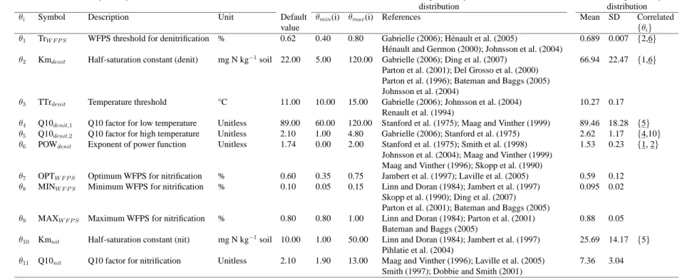
the response functions with the associated parameters are described in Appendix A (Eqs. 7-12).
18
Prior information was gathered on all parameters on a literature review. For lack of information
19
on the form of the pdf of these parameters, the latter were assigned uniform distributions within
20
their likely range derived from literature data (Table 1). Parameters were supposed to be en-
21
tirely independent (i.e. non-correlated). This type of hypotheses, which are likely to be violated
22
in ecosystem models, is not a significant issue in the application of Bayesian calibration. For
1
example, Naud et al. (2007) tested different levels of correlation of prior distributions and con-
2
cluded that correlation was not a very important factor. In addition, Hong et al. (2005) reported
3
that the assumption of a priori independence does not imply independence a posteriori, and the
4
calibration may still provide a posterior estimate of correlations across parameters.
5
2.2 The database of N
2O measurements
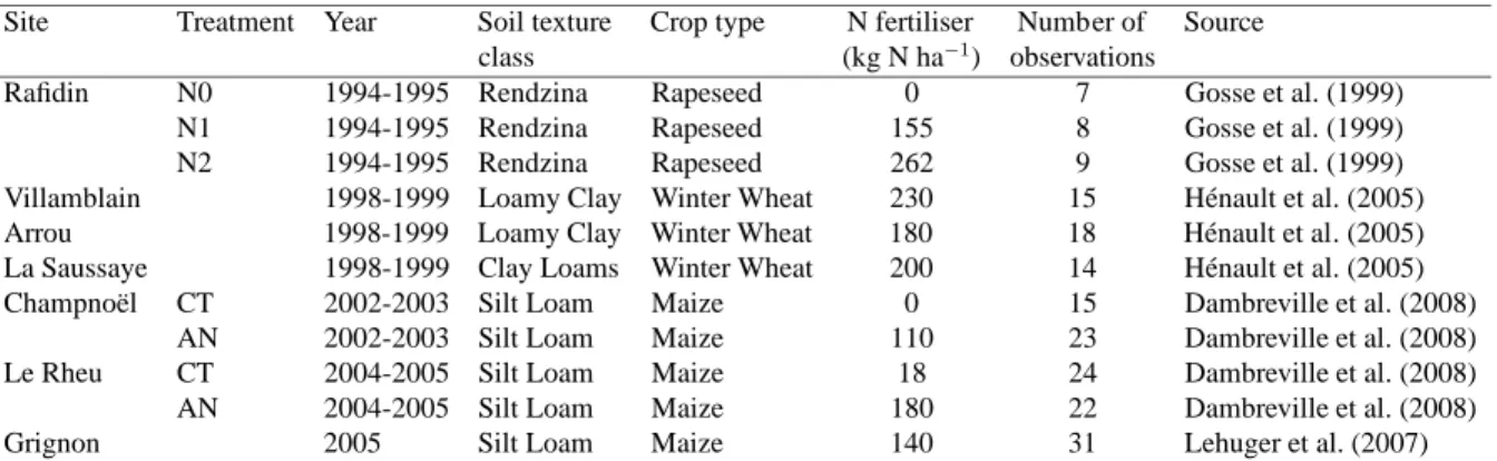
6
The N2O measurements were carried out on seven experimental sites located in Northern France.
7
The experiments were conducted on major arable crop types and soils types representative of
8
this part of France. For some sites, different treatments were conducted with various N-fertiliser
9
amounts supplied to the crop, giving a total of 11 site/treatment combinations (Table 2). Nitrous
10
oxide emissions were monitored by the static chamber method with eight replicates for all sites
11
(H´enault et al., 2005), except at Grignon where measurements were monitored with three auto-
12
matic chambers during 31 successive days from 13 May 2005 to 12 June 2005 (Lehuger et al.,
13
2007). The variance in the measurements was estimated as the variance across the different
14
replicate chambers in the field. Soil nitrogen and moisture contents were monitored in the soil
15
profile for each site with different sampling frequencies (see references of Table 2 for details).
16
The resulting samples were analysed for moisture content and inorganic N using colorimetric
17
samples in the laboratory. Soil temperature was continuously monitored using thermocouples in
18
most of the sites, except for the sites of Champno¨el and Le Rheu. The input data required to run
19
the model were also collected in each site: the weather data were taken from a local meteorolog-
20
ical station, and detailed information on soil properties and crop management were compiled to
21
generate CERES-EGC input files using a standard parameterization procedure (Gabrielle et al.,
22
2006b). Uncertainty on these input data was not considered here since CERES-EGC had already
23
been tested in most of the sites (Gabrielle et al., 2006b). Besides, it likely had little impact on
24
the N2O simulations since we checked that the model gave correct predictions of the major N2O
1
drivers (topsoil environmental conditions and nitrate content).
2
2.3 Bayesian calibration
3
2.3.1 Markov Chain Monte Carlo
4
Bayesian methods are used to estimate model parameters by combining two sources of infor-
5
mation: prior information about parameter values and observations on output variables. The
6
prior information is based on expert knowledge, literature review or by measuring parameters
7
directly in the field or laboratory. In our case, the observations on output variables are field mea-
8
surements of the different fluxes between soil-crop-atmosphere compartments. Bayes’ theorem
9
makes it possible to combine the two sources of information in order to calibrate the model pa-
10
rameters. The first step is to assign a probability distribution to the parameters, representing our
11
prior uncertainty about their values. In our case, we specified lower and upper bounds of the pa-
12
rameters uncertainty, defining the prior parameter distributions as uniform. The aim of Bayesian
13
calibration is to reduce this uncertainty by using the measured data, thereby producing the poste-
14
rior distribution for the parameters. This is achieved by multiplying the prior with the likelihood
15
function, which is the probability of the data given the parameters. The likelihood function is
16
determined by the probability distribution of errors in observations. We assumed errors to be
17
independent and normally distributed with mean zero following Van Oijen et al. (2005) and in
18
the same fashion as Svensson et al. (2008) and Klemedtsson et al. (2007). Because probability
19
densities may be very small numbers, rounding errors needed to be avoided and all calculations
20
were carried out using logarithms. The logarithm of the data likelihood is thus set up, for each
21
data set Yi, as follows:
22
logLi =
K
X
j=1
−0.5
yj −f(ωi;θi) σj
2
−0.5log(2π)−log(σj)
!
(4)
where yjis the mean N2O flux measured on sampling date j in the data set Yi andσj the standard
1
deviation across the replicates on that date, ωi is the vector of model input data for the same
2
date, f(ωi;θi) is the model simulation of yj with the parameter vector θi, and K is the total
3
number of observation dates in the data sets. To generate a representative sample of parameter
4
vectors from the posterior distribution, we used a Markov Chain Monte Carlo (MCMC) method:
5
the Metropolis-Hastings algorithm (Metropolis et al., 1953) (see Appendix B for details). We
6
formed Markov chains of length 104-105using a multivariate Gaussian pdf to generate candidate
7
parameter vectors. The variance matrix of this Gaussian was tuned so that the Markov chains
8
would explore parameter space efficiently. We followed the procedure of Van Oijen et al. (2005)
9
and defined the variances equal to the square of 1 to 5 % of the prior parameter range (θmin-θmax)
10
and zero covariances. Subsequently, the variances were tuned so that the fraction of candidates
11
accepted during the random walk was between 20 to 30%. Ten percent of the total number
12
of iterations at the beginning of the chain were discarded as unrepresentative “burn-in” of the
13
chains (Van Oijen et al., 2005). For each calibration, three parallel Markov chains were started
14
from three different starting points (θ0): the default parameter value and their lower and upper
15
bounds (θminandθmax). Convergence was checked with the diagnostic proposed by Gelman and
16
Rubin (1992), which is based on the comparison of within-chain and between-chain variances,
17
and is similar to a classical analysis of variance. Convergence is reached when variance between
18
chains no longer exceeds the variance within each individual chain. The chains of parameter
19
values resulting from the random walk of the Metropolis-Hastings algorithm are auto-correlated
20
because each iteration depends on the previous one. We therefore thinned the chains in two
21
steps: the auto-correlation was first computed for increasing lags and then the posterior chain
22
was extracted by keeping the iterations defined by the thinning interval. We defined this as the
23
number of iterations between consecutive samples in a chain for which the auto-correlation was
24
less than 60%. The chains filtered in this way were considered to be a representative sample from
25
the posterior pdf, and from this sample were calculated the mean vector, the variance matrix and
1
the 90% confident interval for each parameter.
2
The generation and analysis of the Markov chains were carried out with the statistical package
3
R (R Development Core Team, 2008) and in particular its coda package (Plummer et al., 2006).
4
The CERES-EGC model was encapsulated within R as a library, generated from the original
5
Fortran code.
6
2.3.2 Procedure for the N2O module
7
The calibration procedure had two main objectives: (i) to calibrate the parameters for each dataset
8
Yi, to explore the variations of global parameters across experimental sites and treatments, and
9
(ii) to obtain better estimates for the global parameters (initially deemed universal in the model).
10
The first objective was pursued by calibrating the parameters for each data set separately, which is
11
referred to later on as the dataset-by-dataset procedure. In a second step, the global parameters
12
were calibrated by running our procedure with the 11 data sets simultaneously (multi-dataset
13
procedure), i.e. by calculating the posterior distribution as:
14
p(θ|Y1, ..., Y11)∝p(Y1, ..., Y11|θ)p(θ) (5) where Yi is the data of the ith site and the∝ symbol means ’proportional to’. In this case, the
15
log-likelihood is calculated as the sum of the log-likelihoods of all the data sets (for a given
16
parameter set in the MCMC chain).
17
2.4 Evaluation of model predictions
18
The performance of the calibration procedures was assessed by calculating the root mean square
19
error (RMSE). RMSE was defined, for each data set Yi, as follows (Smith et al., 1996):
20
RM SE = s
PK
j=1(yj−f(ωi;θi))2
K (6)
In both following cases, simulations f(ωi;θi) were carried out using either the posterior ex-
1
pectancy of parameters (θ) or the maximum a posteriori (MAP) estimate of θ (θM AP). θM AP
2
is the single best value of the parameter vector in each MCMC chain, at which the posterior
3
probability distribution is maximal (Van Oijen et al., 2005). In the case of prior parameter pdfs,
4
the simulations were defined as the prior expectancy of the model predictions in which parame-
5
ters were randomly drawn from the prior pdfs. For the posteri or parameters pdfs, the simulations
6
were the posterior expectancy of predictions. RMSE was computed after calibration resulting
7
from the dataset-by-dataset or multi-dataset procedure.
8
3 Results
9
3.1 Simulation of soil state variables
10
Soil temperature, soil water content and nitrate and ammonium contents were simulated by the
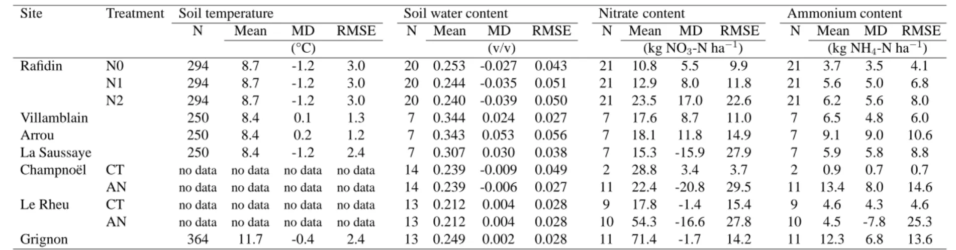
11
model and confronted against the measurements. Table 3 summarizes the mean deviation (MD),
12
which is the mean difference between measurement and simulation, and RMSEs computed with
13
the different topsoil state variables used as input variables of the N2O emission module. Soil
14
temperature and water content were well predicted by the model with RMSE ranging from 1.2
15
to 3.0 ° C for the soil temperature and from 3 to 6 % (v/v) for the soil water content across the
16
11 sites and treatments. The model’s RMSE over the 11 sites and treatments ranged between
17
3.7 to 27.9 kg N ha−1 for the prediction of nitrate content and to 0.7 to 25.3 kg N ha−1 for the
18
ammonium content. Dynamics of surface nitrate and ammonium contents were mainly driven by
19
the fertiliser applications and mineralization of crop residues. Ammonium was rapidly nitrified
20
across all the sites but the model failed to reproduce the background topsoil ammonium stock.
21
Nitrate content was relatively well simulated except for 3 treatments for which N plant uptake
22
was under-estimated (La Saussaye, Champno¨el AN and Le Rheu AN).
23
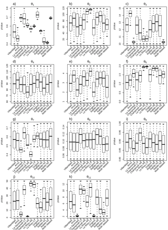
3.2 Posterior parameter distributions
1
Figure 1 shows boxplots of the posterior parameter distributions after calibration with the dataset-
2
by-dataset and the multi-dataset procedures. Such representation makes it possible to visualize
3
differences between parameter pdfs across datasets, while the shape of the boxplot reveals the
4
dispersion and symmetry of the marginal distributions. Our Bayesian procedure generally gen-
5
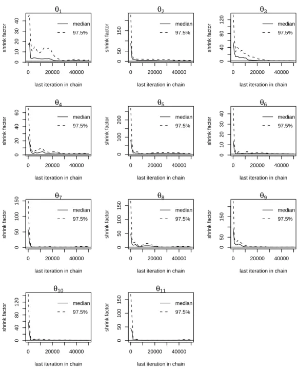
erated uni-modal distributions, and convergence test corroborated that the MCMC chains con-
6
verged. Figure 2 presents the 50 and 97.5% quantiles of the Gelman-Rubin shrink factor for the
7
11 parameters calibrated with the data set of La Saussaye, and shows that it approached 1 for all
8
parameters, evidencing the convergence of the calibration.
9
Figure 1 shows that the posterior distributions became narrower compared to the uniform prior
10
distributions, which is undoubtedly due to the efficiency of our calibration procedure. The pos-
11
terior pdfs converged to normal or log normal distributions, as already observed by Svensson
12
et al. (2008) in the Bayesian calibration of a process-based forest model. Thus, the choice of
13
an uniform distribution for the prior pdfs had little influence, as the information contained in
14
the experimental data gradually became dominant in the calibration process (Van Oijen et al.,
15
2005). For example, the posterior distributions of parameterθ1 (the WFPS threshold triggering
16
denitrification) had a narrow range for all datasets, suggesting that the calibration had drastically
17
reduced its uncertainty. On the contrary, parameters θ8 andθ9 (corresponding to the minimum
18
and maximum WFPS for nitrification activity, respectively) remained spread across their prior
19
range of variation, and centered around their prior median. This means that the calibration did
20
not significantly reduce their uncertainty. Conversely, some posterior distributions were flattened
21
on one of the prior bounds, implying that their optimal values was outside the prescribed range.
22
This was particular true for parameters θ10(the half-saturation constant of nitrification response
23
to ammonium) andθ11 (the Q10 factor for nitrification) for the data sets of Champno¨el AN, La
24
Saussaye and Grignon. We should therefore reconsider the prior ranges for these parameters.
25
The rightmost boxplot in each of the 11 graphs in Figure 1 depicts the distribution obtained with
1
the multi-dataset procedure. The shape of this boxplot and its median value appeared to be more
2
constrained by certain datasets than others, which may be explained by the fact that data sets
3
with a comparatively larger number of observations of higher precision had substantially more
4
weight in the log-likelihood function. For example, the boxplots of the multi-dataset calibration
5
exhibited high similarity with those of the La Saussaye site for parameters θ1,θ3 andθ6.
6
Some data sets were collected in the same sites, i.e. under identical climate patterns and soil
7
types but with differentiated crop management (the Rafidin, Le Rheu and Champno¨el datasets).
8
Since the parameters of the N2O module are mostly related to soil properties, it was expected
9
that the calibration should produce similar distributions for these three sites. To a certain extent,
10
this was the case for the parameters θ2, θ3 and θ6, giving support to the idea that these param-
11
eters are mostly soil-dependent, and are little influenced by crop management. Conversely, the
12
strong variation of posterior pdfs across sites challenges the original idea in model development
13
that these parameters may be considered constant. The purpose of the multi-dataset procedure
14
sought to investigate this option, by seeking the best-fit parameter pdfs in relation to the en-
15
semble of the experimental situations collated in our database. It could be expected to lead to
16
parameter pdfs with a wider spread (and thus higher uncertainty) than in the dataset-by-dataset
17
calibration, owing to the wide ranges covered by the dataset-specific pdfs. While this was true
18
of some parameters (e.g.,θ4,θ5, andθ7), it was the opposite for others (most notablyθ1 andθ3).
19
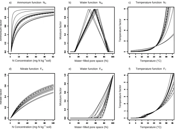
Figure 3 depicts the ranges of response functions of the N2O emission module resulting from the
20
various calibrations, and evidences ample differences across datasets. The responses of nitrifi-
21
cation to soil ammonium content (NN, Fig. 3.a) were highly variable, reflecting the range taken
22
by their shape parameterθ10. The response of nitrification to soil WFPS (NW, Fig. 3.b) shows
23
that the minimum WFPS for nitrification activity (θ8) were centred on a unique value, while the
24
optimum WFPS (θ7) was lower in the calibration with two data sets. The calibrated maximum
25
WFPSs for nitrification (θ9) were centred on 90%. The shapes of the response function NT (Fig.
1
3.c) were similar for two sites (La Saussaye and Grignon), but strikingly different for the other
2
sites. The calibrated responses of denitrification to nitrate content (FN, Fig. 3.d) were highly
3
variable such as the response of nitrification to ammonium content. The shapes of the response
4
of denitrification to WFPS (FW) varied widely, as a consequence of the large variations of param-
5
etersθ1 (the WFPS threshold triggering denitrification) and θ6 (the exponent of the power-law).
6
H´enault and Germon (2000) and Heinen (2006) showed that denitrification was highly sensitive
7
to θ1, and that this parameter was dependent on soil type. The response of denitrification to
8
soil temperature (FT) had a similar shape across the various parameterizations, for temperatures
9
lower than 25 °C which corresponds to the range encountered in the field experiments. This
10
leads to the conclusion that the function calibrated with the multi-dataset procedure could be
11
considered universal.
12
Bayesian calibration also quantifies correlations between parameters in the posterior. Most pa-
13
rameters were cross-correlated, with coefficients higher than 0.4 for 6 of them (Table 1) suggest-
14
ing that our uncertainty about their values is linked and implies that some parameters should be
15
treated in clusters, as suggested by Svensson et al. (2008). Parameters θ1 andθ2 are positively
16
correlated, and are both negatively correlated with θ6.
17
3.3 Model prediction uncertainty
18
The simulations of N2O emissions generated with the posterior MCMC parameter chains pro-
19
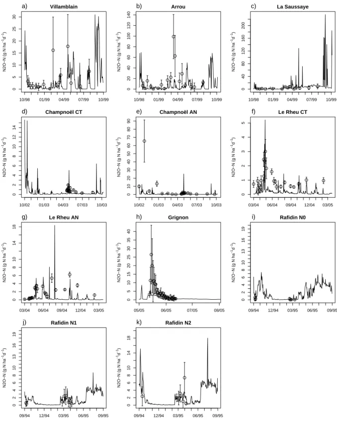
vided statistical distributions of model outputs resulting from parameter uncertainty, which is
20
a straight benefit of Bayesian approaches. Figure 4 shows the mean of simulated daily N2O
21
emissions for all datasets (Fig. 4.a to 4.k). Some discrepancies between measurements and sim-
22
ulations remained, due to uncertainty on both sides. Measurement points with high standard
23
deviations had less weight in the log likelihood function, and thus in the posterior probability,
24
compared to lower fluxes with lower variability. For example, the two N2O spikes measured in
1
Villamblain in springtime (Fig. 4.a) had a large experimental error, but did not appear to con-
2
strain the calibration as much as the more frequent lower N2O fluxes with much lower standard
3
deviations. The same remark applies to Arrou (Fig. 4.b). For the dataset of Champno¨el AN (Fig.
4
4.e), a high spike of N2O was observed in autumn that the model failed to predict, whereas it
5
otherwise successfully simulated fluxes under 10 g N2O-N ha−1d−1.
6
For the Grignon site (Fig. 4.h), the observation points were concentrated on 31 successive days
7
(from 13 May 2005 to 12 June 2005), and started a peak flux. With its default parameter set,
8
the model simulated that peak along with two others in the following weeks that were not ob-
9
served in the field (results not shown, see Lehuger et al. (2007)), in response to significant rains.
10
The Bayesian calibration managed to circumvent the simulation of these two unobserved peak
11
fluxes by raising the WFPS threshold for denitrification (θ1) from 62% (default value) to 73%,
12
which is the highest value in all the calibrations (Fig. 1.a). As a result of this change in the
13
response to rainfall and soil water content, no N2O-peaks were simulated throughout the year
14
in Grignon (Fig. 4.h). For the dataset of Rafidin N0 (Fig. 4.i), observations also were concen-
15
trated on two short periods, but with fewer observations points than at Grignon. The calibration
16
highly constrained the model during the measurement period, but appeared less constraining on
17
the N2O-fluxes outside this period.
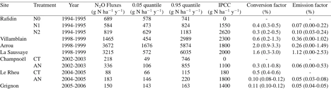
18
Table 4 summarises the statistics of the annual N2O emissions predicted by CERES-EGC for
19
the different datasets. The mean annual fluxes ranged between 88 and 3672 g N2O-N ha−1 y−1,
20
with a large confidence interval especially for the datasets with higher emission rates. An overall
21
conversion factor of fertilizer inputs to N2O-N was calculated as the ratio of the annual flux to the
22
N fertiliser dose. This is different from an “emission factor”, which takes background emissions
23
of N2O into account. Here, we also calculated this factor as the difference between the annual
24
N2O-N emissions of fertilised and unfertilised crops (g N2O-N ha−1y−1) to the N-fertiliser dose.
25
The emission factors ranged from 0.05 and 1.12% across experimental sites, with a mean value
1
of 0.26%. This value is four times lower than the default value recommended by the IPCC tier 1
2
methodology (IPCC, 2006).
3
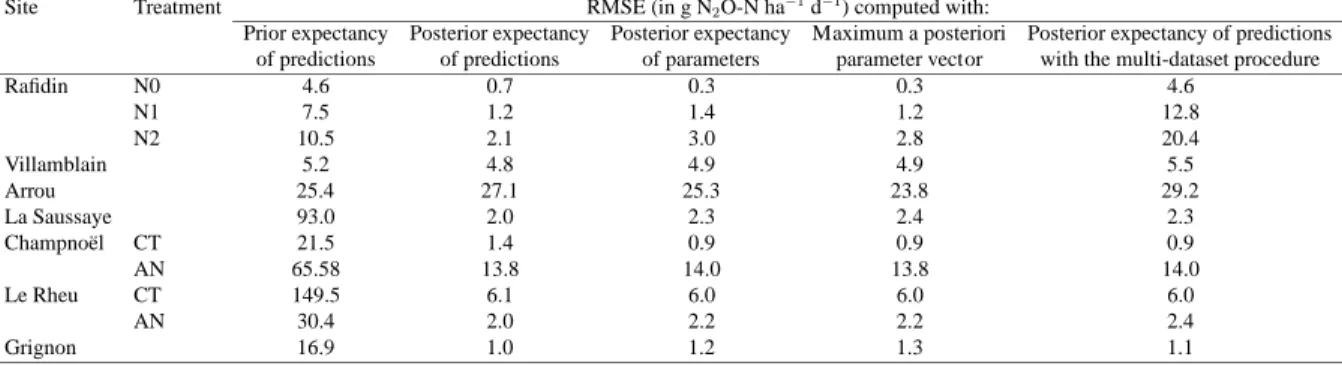
3.4 Calibration efficiency and model prediction error
4
Table 5 summarises the RMSEs obtained with the various parameters sets, and made it possi-
5
ble to compare the efficiency of model calibration whether in the dataset-by-dataset or in the
6
multi-dataset mode. In the dataset-by-dataset procedure, the RMSEs computed with the pos-
7
terior expectancy of predictions were lower than those computed with the prior expectancy of
8
predictions for all datasets except one (Arrou), with a 73% reduction on average and a maxi-
9
mum of 98% in La Saussaye. In 8 of the remaining 9 datasets, calibration lead to a reduction
10
of 79% to 96% in the model’s RMSE. On average across all datasets, the RMSE dropped from
11
39 down to 6 g N2O-N ha−1 d−1after calibration. There were no differences in the RMSEs cal-
12
culated either with simulations based on the posterior mean of parameters (θ) or with posterior
13
mean of predictions. Thus, the mean of our sample from the posterior could be directly used for
14
the sites of our database or for sites with similar soil types. The use of the parameter set with
15
maximum posterior probability (θM AP), i.e. when likelihood was maximum and given that we
16
used a uniform prior, logically improved the RMSE compared to the use of the posterior mean
17
of parameters (θ). As could be expected, the multi-dataset calibration was less efficient than the
18
dataset-by-dataset one, enabling a decrease of only 33% of the RMSE computed with posterior
19
expectancy of predictions compared to the prior expectancy of predictions. This would lead us
20
to believe that the parameter set summarised in Table 1 could be a good compromise when the
21
model will be applied for a new site.
22
In addition, Table 5 shows that the calibration did not really improve the simulations for two
23
datasets: Villamblain and Arrou. For both datasets, the data were not informative enough to
24
significantly improve parameter estimation. In the case of Arrou, the discrepancies may also
1
be explained by the poor ability of CERES-EGC to simulate water-logging effects, as observed
2
in this experiment. The N2O module and in particular its denitrification part (Eqs. 1, 7, 8, 9 -
3
Appendix A) were already shown unable of correctly rendering the dynamics of denitrification
4
or N2O emissions for soils with high degrees of water saturation. Still, RMSE values quantify
5
the mismatch between simulations and the mean of the measurements without taking measure-
6
ment uncertainty into account, or diagnosing whether problem lies with the simulations or the
7
data. As a consequence, RMSE values should be interpreted with caution. More in-depth model
8
evaluation would require comparing the behaviour of multiple models.
9
4 Discussion
10
4.1 Suitability and benefits of Bayesian calibration
11
Our main goal was to demonstrate the potential of a Bayesian-type calibration procedure to im-
12
prove the parameterization of a N2O-emission model, quantify parameter uncertainty and reduce
13
uncertainties of model outputs. In recent years, Bayesian calibration was successfully applied to
14
process-based ecosystem models, such as forest biomass growth models (Van Oijen et al., 2005;
15
Svensson et al., 2008; Klemedtsson et al., 2007). Among the various possible Bayesian methods,
16
MCMC is in principle particularly well adapted to such models (and in particular CERES-EGC)
17
because they can handle a high number of parameters simultaneously (Makowski et al., 2002).
18
Their efficiency is also not hampered by a poor knowlegde of the prior distributions, as is often
19
the case with this type of models, and may be judged from the large variation range of the param-
20
eters we calibrated here. Method of expert elicitation have been recently developed and could
21
be used in the future in order to refine prior distributions of model parameters. In short, elicita-
22
tion is the process of translating expert knowledge about uncertain quantities into a probability
23
distribution (Oakley and O’Hagan, 2007). However, no attempts had been made yet to calibrate
24
processes so uncertain and irregular in time and space as N2O emissions. This raised a number
1
of issues in the adaptation of the MCMC algorithm. In particular, the chains were strongly auto-
2
correlated, which required a substantial number of iterations (104 to 105), and drastic thinning.
3
Also, the convergence had to be tested by running three parallel chains and using a variance-based
4
diagnostic. An accurate simulation of the soil environmental drivers (temperature, moisture and
5
mineral N contents) was a pre-requisite for the prediction of N2O fluxes. Tests against field
6
data showed that this condition was overall met, as noted in a previous test of CERES-EGC in a
7
subset of the sites used here (Gabrielle et al., 2006b). In some instances, some discrepancies in
8
the simulation of topsoil water content (Arrou) or nitrate content (La Saussaye, Champno¨el AN
9
and Le Rheu AN) which affected the prediction of N2O fluxes. However, these errors point to
10
structural deficiencies of the model (for instance in the simulation of soil water dynamics in the
11
water-logged soil of Arrou), and did not interfere with the calibration. This was evidenced by
12
the fact that inclusion of measured drivers improved model performance only marginally and in
13
a few sites. This option was thus disregarded.
14
Our procedure significantly reduced parameter uncertainty for the datasets, and the uncertainty
15
in simulated N2O rates as a result. We have also established a database of N2O emissions for
16
Northern France and in the future, it will be interesting to use this one to parameterise other mod-
17
els or to compare the performance of different N2O emissions process-based module integrated
18
in CERES-EGC. Another direction could also be to use other kind of output data to parameterise
19
specific module, for example the use of NO emission measurements for calibration of the nitri-
20
fication sub-module (Eqs. 2, 10, 11, 12) of CERES-EGC (Rolland et al., 2008). The procedure
21
we successfully implemented here may be readily used for other components of CERES-EGC,
22
such as soil C turnover or crop photosynthesis and growth.
23
The calibration significantly reduced the model’s RMSE compared with the prior parameter val-
24
ues, on average by 73% with the data-by-dataset procedure and by 33% with the multi-dataset
25
procedure. Still, the calibration did not result in a perfect match between model simulations and
1
observations of the daily N2O fluxes. Measured data with high uncertainty were in particular
2
less well predicted because they presented a high spatial variability and consequently were less
3
constraining in the calculation of the likelihood function. This may also be seen as an advantage
4
since these extreme data points with large variance did not artificially influence the parameter
5
values compared to lower-range values with better accuracy. Heinen (2006) also showed with a
6
different calibration method that the optimised denitrification sub-module did not result in per-
7
fect fit at the daily compared to the seasonal scale.
8
Lastly, the dataset-by-dataset calibration points to ways of optimising calibration efficiency:
9
when using manual chambers, N2O measurements should be carried out at least once a month
10
throughout the year, with a higher frequency during the peak fluxes subsequent to N-fertiliser
11
and crop residues inputs and when soil conditions are favourable to denitrification , e.g. when
12
soil moisture, soil temperature and mineralization rate are high.
13
4.2 Spatial variability of model parameters
14
We sought to calibrate model parameters either on a dataset-by-dataset basis in order to minimise
15
model error or simultaneously on all datasets to find parameter values that would be universally
16
applicable, following the premise behind the original development of the N2O model. Such
17
values would be extremely useful to apply the model to new soil conditions and to spatially
18
extrapolate it. However, it was suggested that simple process-based models such as the one we
19
used here needs to be parameterised on a site-specific basis (Heinen, 2006). The latter authors
20
concluded to the impossibility of defining a set of response functions for denitrification (Eqs 1, 7
21
,8, 9 - appendix A) that would equally apply to sandy, loamy and peat soil types. Our dataset-by-
22
dataset calibration gave further evidence to that statement for the N2O module of CERES-EGC,
23
judging from the large variations in parameter pdfs across sites. However, our multi-dataset
24
procedure also demonstrated that it is still possible to find global estimates for those parameters
1
that encompass a wide range of experimental conditions, at the cost of a higher RMSE than
2
with optimal, site-specific parameter sets. The parameter pdfs we obtained in the multi-dataset
3
calibration shows which parameter values would be plausible, and may thus be used to improve
4
the accuracy of N2O simulations in new sites.
5
Models are often developed with the purpose of providing predictions over a large domain (in
6
space and time). However, ensuring that their parameterisation is accurate is a pre-requisite to
7
such application. When attempting at simulating N2O fluxes in a new site where no measured
8
data are available, the results of our calibration points to the following strategy to meet this
9
requirement. First, the user should check if calibrated parameter sets already exist for similar
10
soil types, based on soil taxonomy or physico-chemical characteristics. If not, the parameter
11
values derived from the multi-dataset calibration may be used. They may also serve as default
12
values for the spatial extrapolation of the model at the regional scale. In the future, new data
13
sets may be assimilated in the calibration to reduce the uncertainty of global parameters and to
14
increase the application domain of the model. Alternatively, it is clearly advisable to favour the
15
collection of N2O emissions data for the new sites, which lead to a much better performance
16
of the model. One last obstacle to the extrapolation of CERES-EGC lies in the 4 site-specific
17
parameters, which are supposed to be measured in the laboratory. We chose to exclude them from
18
the calibration in accordance with the original model design. However, including them would be
19
interesting to simulate a situation where such experimental determination is not possible, and to
20
see to what extent it influences the outcome of the calibration. It is likely to result in different
21
parameter values since, for instance, the potential denitrification rate (a local parameter) was
22
shown to significantly correlate with three global parameters related to denitrification (Gabrielle,
23
2006). However, testing such a scenario appeared beyond the scope of this paper since it implied
24
too strong a deviation from the model hypotheses.
25
4.3 Prediction of N
2O fluxes from agro-ecosystems
1
CERES-EGC and its specific N2O module have already been used in a range of soil conditions
2
(H´enault et al., 2005; Dambreville et al., 2008; Heinen, 2006), and model uncertainty had only
3
been quantified using simple Monte Carlo techniques for a subset of 5 parameters (Gabrielle
4
et al., 2006a). The effect of parameter uncertainty was seldom analysed with ecosystem models
5
simulating N2O emissions, although (or perhaps also because) N2O measurements are fraught
6
with a daunting spatial and temporal variability (Duxbury and Bouldin, 1982). Our Bayesian
7
calibration resulted in a probabilistic simulation of the time course of N2O emissions taking
8
such variability and uncertainty into account, through their consequences on parameters’ distri-
9
butions. The calibrated model could predict daily N2O fluxes rather well, except for the highest
10
peaks with high experimental error which it failed to predict in some cases.
11
In addition, the procedure makes it possible to quantify model output uncertainty in the calcula-
12
tion of annual N2O budget and emission factors (EFs). The model predicted annual N2O fluxes
13
were ranging from 88 to 3672 g N2O-N ha−1y−1 over the various sites, and EFs ranging from
14
0.05 to 1.12%. On the basis of these results, alongside those of Gabrielle et al. (2006a), it ap-
15
pears that the 1% default EF value of the IPCC Tier 1 methodology is not suitable for the sites we
16
studied because it would considerably overestimate the annual emissions (Table 4). In Belgium,
17
Beheydt et al. (2007) used the DNDC model to calculate EFs corresponding to various scenarios
18
involving high N input levels and N surpluses, and obtained an average value of 6.49%, which
19
is 25 times higher than ours, compared to an estimate of 3.16% using the N2O measurements.
20
Their observed emission range was an order of magnitude higher than that of our database. As-
21
similate such extreme data with our procedure would be helpful to enlarge the prediction range
22
of CERES-EGC, and to check its ability to predict annual emissions higher than 10 kg N2O-
23
N ha−1 y−1.
24
Our results also suggested that annual N2O emissions were not strictly proportional to fertiliser
25
N rate, which is in agreement with the results of Barton et al. (2008). The latter showed that,
1
in a semi-arid climate, in spite of the application of N fertiliser the annual N2O emissions were
2
not significantly increased in comparison with background emissions. They concluded that the
3
emissions of N2O from arable soils could not be directly derived from the application of N fer-
4
tiliser, and that other factors (e.g., soil properties) should be taken into account.
5
Bayesian calibration provided valuable insight into the uncertainty of the simulated N2O fluxes,
6
making it possible to take risk into account in a range of model applications: estimation of the
7
global warming potential (GWP) of agro-ecosystems, assessment of cropping systems’ environ-
8
mental balance, or decision support in agriculture. It would also be interesting to compare the
9
ability of various agro-ecosystem models to predict N2O emissions on the same data sets, in a
10
similar fashion as Frolking et al. (1998) and Li et al. (2005). Furthermore, Bayesian Model Com-
11
parison (Van Oijen et al., 2005; Kass and Raftery, 1995) could be applied to examine multiple
12
models and to quantify their relative likelihood, i.e. by determining which model is most prob-
13
able in view of the data and prior information. Finally, the outputs of several models could be
14
combined to improve the accuracy of the prediction, as was suggested with atmospheric models
15
(Fisher et al., 2002).
16
5 Conclusion and future work
17
Bayesian calibration was successfully applied to the CERES-EGC agro-ecosystem model to im-
18
prove the parameterization of its N2O emission module, thanks to a careful analysis and diag-
19
nostic of the MCMC chains of parameters generated by the Metropolis-Hastings algorithm. The
20
parameters were calibrated either (i) against separately data sets or (ii) by using all the data sets
21
simultaneously, to satisfy our objectives which were, respectively, to improve model simula-
22
tions at the field scale and to find universal values of parameters in order to spatially extrapolate
23
the model. In addition, Bayesian calibration provided a means of quantifying uncertainties in
24
both parameters and model outputs. Furthermore, it appears reasonable to assume that when the
1
model should be applied at a larger scale than the plot-scale, the parameter values resulted from
2
the multi-dataset procedure could then be used for soil types which will have never been parame-
3
terised. In fact, the posterior parameter distributions encompass all our current observations and
4
give us the possibility of quantifying their uncertainty.
5
A remaining obstacle to the extrapolation of the N2O module lies in the 4 local parameters that
6
should be measured or estimated on site (H´enault et al., 2005), and that were accordingly not
7
calibrated here. Identifying the key soil or landscape characteristics that control these parame-
8
ters appears as a pre-requisite to the large-scale use of CERES-EGC.
9
Based on our results, we recommended a strategy to deal with model extrapolation and parame-
10
ters’ variability. Nevertheless, another option to tackle spatial variability would consist in using
11
other types of prior information (e.g. on soil properties) to infer the parameters of the N2O mod-
12
ule. In future work, it would be beneficial to identify such “hyperparameters” which may explain
13
spatial variability (Clark, 2005), and to develop a hierarchical Bayesian approach to derive their
14
pdfs.
15
Acknowledgements
16
This work was part of the NitroEurope Integrated Project (EU’s Sixth Framework Programme for
17
Research and Technological Development) which investigates the nitrogen cycle and its influence
18
on the European greenhouse gas balance. We wish to thank Matieyiendu Lamboni and Herv´e
19
Monod (INRA Jouy-en-Josas) for useful advice and discussions. Special thanks to Christophe
20
Dambreville for making available the data from the Champno¨el and Le Rheu sites.
21