[PENDING] A Cartesian Cut Cell Method for Rarefied Flow Simulations around Moving Obstacles

HAL Id: hal-01131756

https://hal.archives-ouvertes.fr/hal-01131756

Submitted on 15 Mar 2015

HAL is a multi-disciplinary open access archive for the deposit and dissemination of sci- entific research documents, whether they are pub- lished or not. The documents may come from teaching and research institutions in France or abroad, or from public or private research centers.

L’archive ouverte pluridisciplinaire HAL, est destinée au dépôt et à la diffusion de documents scientifiques de niveau recherche, publiés ou non, émanant des établissements d’enseignement et de recherche français ou étrangers, des laboratoires publics ou privés.

A Cartesian Cut Cell Method for Rarefied Flow Simulations around Moving Obstacles

Guillaume Dechristé, Luc Mieussens

To cite this version:

Guillaume Dechristé, Luc Mieussens. A Cartesian Cut Cell Method for Rarefied Flow Simulations around Moving Obstacles. Journal of Computational Physics, Elsevier, 2016, 314 (1), pp.465-488.

�10.1016/j.jcp.2016.03.024�. �hal-01131756�

A Cartesian Cut Cell Method for Rarefied Flow Simulations around Moving Obstacles

G. Dechrist´e¹, L. Mieussens²

1Univ. Bordeaux, IMB, UMR 5251, F-33400 Talence, France.

CNRS, IMB, UMR 5251, F-33400 Talence, France.

(Guillaume.Dechriste@math.u-bordeaux1.fr)

2Univ. Bordeaux, IMB, UMR 5251, F-33400 Talence, France.

CNRS, IMB, UMR 5251, F-33400 Talence, France.

Bordeaux INP, IMB, UMR 5251, F-33400 Talence, France.

INRIA, F-33400 Talence, France.

(Luc.Mieussens@math.u-bordeaux1.fr) Abstract

For accurate simulations of rarefied gas flows around moving obstacles, we propose a cut cell method on Cartesian grids: it allows exact conservation and accurate treatment of boundary conditions. Our approach is designed to treat Cartesian cells and various kind of cut cells by the same algorithm, with no need to identify the specific shape of each cut cell. This makes the implementation quite simple, and allows a direct extension to 3D problems. Such simulations are also made possible by using an adaptive mesh refinement technique and a hybrid parallel implementation. This is illustrated by several test cases, including a 3D unsteady simulation of the Crookes radiometer.

Keywords: kinetic equations, deterministic method, immersed boundaries, cut cell method, rarefied gas dynamics

1 Introduction

In gas dynamic problems, the rarefied regime appears when the mean free path of the molecules of the gas is of the same order of magnitude as a characteristic macroscopic length. The flow has to be modeled by the Boltzmann equation of the kinetic theory of gases. Most of numerical simulations for rarefied flows are made with the stochastic DSMC method [6], especially for aerodynamical flows in re-entry problems. In the past few years, several deterministic solvers have been proposed, that are based on discretizations of the Boltzmann equation or simplified models, like BGK, ES-BGK, or Shakhov models [28].

They are efficient for accurate simulations, multi-scale problems, or transitional flows, for instance.

A recent issue is the account of solid boundary motion in rarefied flow simulations.

This is necessary to simulate flows around moving parts of micro-electromechanical systems

(MEMS) [17, 23], as well as flows inside vacuum pumps. A fascinating illustration of rarefied flows with moving boundaries is the Crookes radiometer, subject of many debates from the late 19th to early 20th century [24]. Recent deterministic simulations help to understand the origin of the radiometric forces [36, 41, 42, 9]. The numerical simulation of the Crookes radiometer is difficult because the motion of the vanes is induced by gas/solid interaction (like thermal creep), which means that an accurate prediction of the flow in the vicinity of the boundary is needed in order to predict the correct velocity of the vanes.

There are several numerical methods for moving boundary problems designed for com- putational fluid dynamics: some of them have recently been extended to deterministic dis- cretizations of kinetic models, and can be divided in two main categories.

First, with body fitted methods, the mesh is adapted at each time step so that the bound- ary of the computational domain always fit with the physical boundary: moving mesh [43]

and ALE methods [18, 19] fall into this category. Despite their extensive use in computa- tional fluid dynamics, very few similar works have been reported in kinetic theory, except by Chen et al. [10]. Methods of the second category are based on Cartesian grid computations and are usually referred to as immersed boundary methods [29]. The mesh does not change during computations, and hence does not fit with the physical boundary. Special treatment is applied on mesh cells that are located close to the boundary in order to take its motion into account. Various extensions of these methods to kinetic theory have been proposed by several authors in [2, 31, 14, 4]. Two recent variants are the inverse Lax-Wendroff immersed boundary method proposed by Filbet and Yang [16] and the Cartesian grid-based unified gas kinetic scheme of Chen and Xu [8]: the boundary motion is not taken into account in these two works, but these methods could in principle be extended to this kind of problem. We also mention the Lagrangian method: while it falls into the first category in CFD, it does not in kinetic theory. Indeed, whatever the motion of the mesh, the distribution function has to be interpolated at the foot of the characteristic for each microscopic velocity. The accuracy of these methods have been shown in [35, 47] for one dimensional problems. Finally, we mention that moving boundary flows can also be treated with DSMC solvers: see, for instance, [30, 33, 39, 40].

In this paper, we try to mix the advantages of body fitted and Cartesian methods: we present a cut cell method for computing rarefied gas flows around moving obstacles. The cut cell method belongs to the Cartesian grid based methods and has been widely used in computational fluid dynamics [22]. However, this is the first extension to moving boundary problems in kinetic theory (complex 3D stationary DSMC simulations have already been investigated in [26, 48]). This approach is well suited to deterministic approximations of the Boltzmann equation and is easy to implement because of the Cartesian structure of the mesh. Moreover, this is, up to our knowledge, the only immersed boundary method to be conservative. The versatility and robustness of the technique is illustrated by various 2D flows, and by the simulation of the unsteady rotation of the vanes of a 3D Crookes radiometer. This article is an extended version of our work announced in [14]. Here, the Boltzmann collision operator is replaced by BGK like models, which is approximated by a discrete velocity method. However, this is not a restriction: other collision operators could

be used, and any velocity approximation (like the spectral method) could be used.

Generally, the problem of cut cell methods is that it is difficult to take into account the various shapes of cells that are cut by the solid boundary: for instance, in 2D, a cut cell can be a triangle, a quadrangle, or a pentagon, and this is worse in 3D. Here, we propose a simple representation of these cells by using the notion of virtual cells that are polygons (or polyedrals) with possibly degenerated edges (or faces). This makes the treatment of any cut cell completely generic: in the implementation, the different kinds of cut cells and the non cut cells are treated by the same algorithm. This makes the extension of the method to 3D problems very easy. However, to make large scale 3D simulations possible, we also use an adaptive mesh refinement (AMR) technique and a special parallel implementation.

The outline of our paper is as follows. In section 2, we give the governing equations of rarefied gas flows and introduce some notations. Our cut cell method is presented in section 3 for 2D problems. It is validated on three different numerical examples in section 4. Then, in section 5, our algorithm is extended to 3D simulations, and a 3D unsteady simulation of the Crookes radiometer is presented. Finally, some conclusions and perspectives are discussed in section 6. Technical details like computations of geometric parameters of the cells are presented in the Appendix.

2 Rarefied gas dynamics

2.1 Boltzmann equation

In rarefied regimes, a monoatomic gas is described by the Boltzmann equation:

∂F

∂t +~v· ∇F =Q(F). (1)

The distribution functionF(t, ~x, ~v) is the mass density of molecules at timetthat are located at the space coordinate~x∈R³ and that have a velocity~v ∈R³. For our approach, it is more relevant to look at the integral form of (1) in a time dependent volumeV(t). The Reynolds transport theorem leads to:

∂

∂t Z

V

FdV + Z

∂V

(~v−w)~ ·~nFdS = Z

V

Q(F) dV, (2)

where∂V(t) is the surface of the volume V(t). Let~xbe a point of this surface: it is moving at a velocity w(t, ~~ x) and the vector ~n(t, ~x) is the outward normal vector to the surface at this point.

The density ρ, momentum ρ~u, total energy E, stress tensor Σ and heat flux ~q, are

computed by the first moments of the distribution function with respect to the velocity:



 ρ ρ~u

E



= Z

R³



 1 k~vk

1 2k~vk²



F(t, ~x, ~v) dv_xdv_ydv_z, Σ =

Z

R³

(~v −~u)⊗(~v−~u)F(t, ~x, ~v) dvxdvydvz,

~ q=

Z

R³

1

2(~v−~u)k~v−~uk²F(t, ~x, ~v) dv_xdv_ydv_z,

(3)

where the norm is defined by k~vk² =v²_x+v²_y +v_z². The temperatureT of the gas is related to the the energy by the relation E = ¹₂ρk~uk²+³₂ρRT, whereR is the gas constant defined as the ratio between the Boltzmann constant and the molecular mass of the gas. Moreover, the pressure is computed with the standard equation of state for ideal gases: P =ρRT.

When a gas is at rest, which means in equilibrium state, the molecules are uniformly distributed around the macroscopic velocity and the distribution function is a Gaussian function called Maxwellian:

M[ρ, ~u, T](~v) = ρ

(2πRT)^3/2 exp

−k~v−~uk² 2RT

. (4)

The Boltzmann equation implies that the total variation of F comes from the collisions between particles, that are modeled by the Boltzmann operator Q(F). This operator is computationally expensive and several models have been introduced to make its computa- tion easier. Simplest models consists in a relaxation of the distribution function towards a corresponding equilibrium function E:

Q(F) = 1

τ(E −F),

where τ is a relaxation time (see various definitions in section 4). Bhatnagar, Gross and Krook [5] proposed to take E equal to the local equilibrium state, that is

E =M[ρ, ~u, T].

The corresponding BGK model conserves mass, momentum and total energy since the first three moments of the Maxwellian are the same as those of the distribution function. A Chapman-Enskog expansion [7] gives relations between viscosity µ, heat conduction κ and relaxation time. In this case, the expansion yields µ=τ P and κ = ⁵₂R τ P. It may be seen that the BGK model necessarily leads to Prandtl number Pr = ⁵₂µR/κ equal to 1. However for most of gases, it is physically found to be less than this. More complex functions E such that in Holway [20] and Shakhov [38] models have been developed to obtain the correct Prandtl number. For instance, for the Shakhov model, E reads

E =M[ρ, ~u, T]

1 + (1−Pr)(~v−~u)·~q

k~v−~uk²

RT −5

.

(5P RT)

.

In this article, solid wall interactions are taken into account by the standard fully diffuse reflection. This model states that all particles that collide with a boundary are absorbed by the wall and re emitted with a Maxwellian distribution:

F(t, ~x∈Γ, ~v ∈ V_in) = φM[1, ~u_w, T_w], (5) whereT_w and~u_w are the temperature and the velocity of the boundary Γ at position~x. The coefficient φ is computed in order to set the net mass flux across the wall to zero:

φ =− Z

~v∈Vout

(~v−~uw)·~nwF dvxdvydvz

.Z

~v∈V_in

(~v −~uw)·~nwM[1, ~uw, Tw] dvxdvydvz

. The set of incoming velocities is defined by Vin = {~v such that (~v −~uw)·~nw < 0}, where

~n_w is the normal vector to the boundary, pointed to the wall. Similarly, the set of outgoing velocities is V_out = {~v such that (~v −~u_w)·~n_w > 0}. Note that the boundary condition is defined only for the relative incoming microscopic velocities.

2.2 Reduced model

For plane flows, the computational complexity of the Boltzmann equation can be decreased by the use of a standard reduced distribution technique [11]. This classical method has been extensively used for numerical computations of BGK and Shakhov models. First note that in plane flows, the third component of the macroscopic velocity u_z is equal to zero, as well as q_z, Σ_xz, and Σ_yz. From now on, we define the two dimensional variables

x= (x, y), v= (v_x, v_y), u= (u_x, u_y), q= (q_x, q_y), Σ =

Σ_xx Σ_xy Σ_yx Σ_yy

. Letf and g be the reduced distribution functions defined by

f(v) = Z

R

F(~v)dv_z, g(v) = Z

R

1

2v²_zF(~v)dv_z.

The macroscopic quantities can be computed from f and g. Indeed, the set of equations (3) readily becomes



 ρ ρu

E



= Z

R²



 1 v

1 2kvk²



f(v) dv_xdv_y+ Z

R²



 0 0 1



g(v) dv_xdv_y, Σ =

Z

R²

(v−u)⊗(v−u)f(v) dv_xdv_y, q=

Z

R²

(v−u) 1

2kv−uk²f(v) +g(v)

dvxdvy,

(6)

where kvk² = v_x² +v_y². Multiplying by (1,¹₂v²_z) the Boltzmann equation (2) and then inte- grating the result with respect to v_z gives the following set of equations:

∂

∂t Z

S

fdS+ Z

∂S

(v−w)·nfdl= Z

S

1

τ(f−f) dS,

∂

∂t Z

S

gdS+ Z

∂S

(v−w)·ngdl = Z

S

1

τ(g−g) dS.

(7)

In this case, ∂S(t) is the contour of the surface S(t). Each point x∈ ∂S(t) is moving at a velocity w(t, ~x) and n(t, ~x) is the outward normal vector to the contour at this point. The reduced equilibrium functions are defined by

f=M[ρ,u, T] and g = RT

2 M[ρ,u, T], (8)

for the BGK model and by f=M[ρ,u, T]

1 + (1−Pr)(v−u)·q

kv−uk²

RT −4

.

(5P RT)

, g= RT

2 M[ρ,u, T]

1 + (1−Pr)(v−u)·q

kv−uk²

RT −2

.

(5P RT)

,

(9)

for the Shakhov model, where M[ρ,u, T] is the reduced Maxwellian given by M[ρ,u, T](v) = ρ

2πRT exp

−kv−uk² 2RT

.

To close this section, the boundary conditions (5) are written with the reduced distribution functions as:

f(t,x∈Γ,v∈ V_in) = φM[1,u_w, T_w], g(t,x∈Γ,v∈ V_in) =φRT

2 M[1,u_w, T_w], (10)

where φ is computed by φ=−

Z

v∈Vout

(v−u_w)·n_wfdv_xdv_y

.Z

v∈Vin

(v−u_w)·n_wM[1,u_w, T_w] dv_xdv_y

. In this formula, u_w and T_w are the velocity and temperature of the point x that belongs to the boundary Γ, and n_w is the normal vector to the boundary pointed to the wall.

The relative incoming and outgoing velocities at this point are therefore defined by V_in = {v such that (v−u_w)·n_w <0} and V_out ={vsuch that (v−u_w)·n_w >0}.

3 The cut-cell method for two dimensional problems

In this section, we present a numerical method to simulate plane flows with moving bound- aries. The governing equations are detailed in section 2.2. The discretization of each variable (velocity, space, and time) is presented in separate sections.

3.1 Discrete velocity approximation

The velocity space is discretized by a Cartesian grid. Let vmin ∈ R² and vmax ∈ R² be the lower-left and upper-right corners of this grid. The number of discrete velocities is N², the velocity step is denoted by (∆v_x,∆v_y) = (v_max−v_min)/N, and the p^th velocity is vp = vmin + (p1∆vx, p2∆vy), such that p = p2N +p1 for all (p1, p2) ∈ [0, N −1]². The approximation of the distribution function is defined by f_p(t,x) = f(t,x,v_p). The set of equations (7) is discretized with respect to v by the following set of 2N² equations:

∂

∂t Z

S

f_pdS+ Z

∂S

(v_p −w)·nf_pdl= Z

S

1

τ(fp−f_p) dS,

∂

∂t Z

S

g_pdS+ Z

∂S

(v_p−w)·ng_pdl = Z

S

1

τ(gp−g_p) dS.

(11)

The macroscopic quantities are computed with (6), where the integrals overR² are approx- imated by a sum over the N² discrete velocity points. They are therefore given by



 ρ ρu

E



=

N²−1

X

p=0



 1 v_p

1 2||v_p||²



fp∆vx∆vy +

N²−1

X

p=0



 0 0 1



gp∆vx∆vy, Σ =

N²−1

X

p=0

(v_p−u)⊗(v_p−u)f_p∆v_x∆v_y,

q=

N²−1

X

p=0

(v_p−u) 1

2||v_p−u||²f_p+g_p

∆v_x∆v_y.

(12)

Finally, the equilibrium functions fp and gp are computed either with (8) or with (9).

However, the triplet (ρ,u, T) used in these formulas is obtained with a Newton algorithm that preserves the discrete conservation of Boltzmann equation, rather than with direct computation (12) of the macroscopic quantities. Note that instead of using the algorithm of [27] which is based on entropic variables, we use the algorithm of Titarev [45].

3.2 Space discretization

3.2.1 Cartesian grid and cut cells

Let Ω = [xmin, xmax]×[ymin, ymax] denote the space computational domain. It is discretized by a Cartesian grid of (N_x + 1)× (N_y + 1) points. Their coordinates are computed for all (i, j) ∈ [0, N_x]×[0, N_y] by x_i+¹

2,j+¹₂ = x_min + (i∆x, j∆y), where (∆x,∆y) = ([x_max− x_min]/N_x,[y_max−y_min]/N_y) and x_min = (x_min, y_min). The computational mesh is therefore made up by Nx×Ny rectangular cells: each cell is denoted by Ωi,j and its center isxi,j.

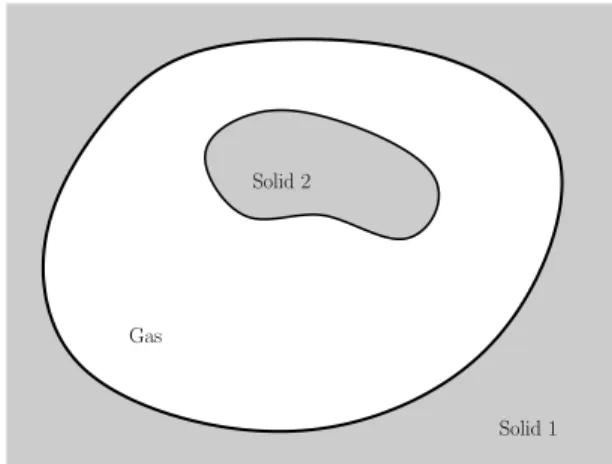
Since the computational domain is rectangular, physical boundaries do not necessarily fit with the mesh boundary. In order to simulate arbitrary shaped objects, solid and gaseous

domains Ω_s(t) and Ω_g(t) are introduced. They correspond to the solid and gaseous parts of the computational domain and hence Ω = Ω_s(t)∪Ω_g(t). We point out that while Ω_s and Ω_g are time dependent, Ω is not. At time t > 0, a rectangular cell Ω_i,j can be in one of these three different states only:

• Ω_i,j is a gas cell if it is completely contained in the gaseous domain: Ω_i,j∩Ω_s(t) =∅.

• Ωi,j is a solid cell if it is completely contained in the solid domain: Ωi,j∩Ωg(t) = ∅.

• Ω_i,jis acut cell if it is partially contained in the gaseous domain and partially contained in the solid domain: Ω_i,j∩Ω_s(t)6=∅ and Ω_i,j∩Ω_g(t)6=∅.

These three states of cells are shown in figure 1.

3.2.2 Virtual cells

To each cell Ωi,j is now associated a virtual cell Ωi,j(t), which is the section of Ωi,j contained in the gaseous domain: this reads Ω_i,j(t) = Ω_i,j∩Ω_g(t). Whatever the state of the cell (that is to say gas, solid or cut), it is defined with five virtual edges, whose lenghts can be zero.

Four of them, that are denoted by L_i±¹

2,j(t) and L_i,j±¹

2(t), fit with the lines of the Cartesian mesh. The last one, denoted by Li,j(t), is a linear approximation of the solid boundary. If the virtual cell has less than five real edges, then at least one length is zero. Finally, we denote by s_i,j the area of the virtual cell, and|L| will denote the length of any edge L.

At a given time tⁿ=n∆t, all these parameters are denoted as follows:

Ωⁿ_i,j = Ω_i,j(tⁿ), Lⁿ_i±1

2,j =L_i±¹

2,j(tⁿ), Lⁿ_i,j±1 2

=L_i,j±¹

2(tⁿ), Lⁿ_i,j =L_i,j(tⁿ), sⁿ_i,j =s_i,j(tⁿ).

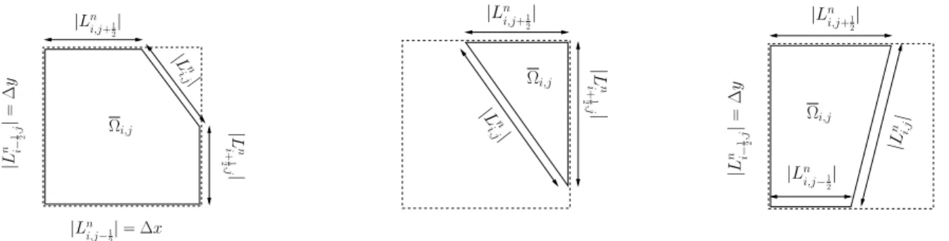
Note that a difficult problem in the cut cell method is that cut cells can take many different shapes (mainly in 3D), which can make the code very complex. A key element of our approach is that all these different shapes are treated generically by using this notion of virtual cell with its 5 virtual edges. Indeed, all the cells are treated in the same way, whatever their state (gas, solid, cut cell) or shape. The different parameters of the three cell states are summarized below, and we refer to figure 2 for three examples of cut cells:

• gas cell: Ωⁿ_i,j = Ω_i,j, |Lⁿ_i±1

2,j|= ∆y,|Lⁿ_i,j±1 2

|= ∆x, |Lⁿ_i,j|= 0, sⁿ_i,j = ∆x∆y,

• solid cell: Ωⁿ_i,j =∅,|Lⁿ_i±1

2,j|= 0, |Lⁿ_i,j±1 2

|= 0, |Lⁿ_i,j|= 0, sⁿ_i,j = 0,

• cut cell: Ωⁿ_i,j is a part of Ω_i,j, and the five lengths of the virtual cell|Lⁿ_i±1

2,j|, |Lⁿ_i,j±1 2

|, and |Lⁿ_i,j| can take any value between 0 and ∆y, ∆x, and p

∆x²+ ∆y², respectively (see figure 2).

All these parameters are computed with a levelset technique, as explained in appendix A.

3.2.3 Control volumes

The notion of control volume is essential to avoid the use of very small virtual cells that would lead to prohibitively small time steps. The idea is to merge small virtual cells with larger neighboring cells when their areas are smaller than half of the area of a Cartesian cell.

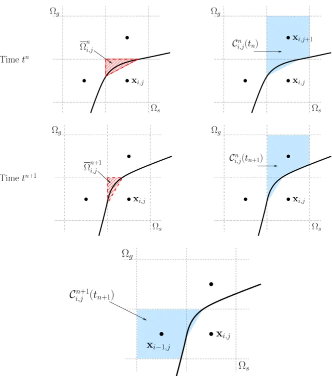
The control volume is constructed by recursion: we look at a given cut cell Ωi,j whose center is inside the solid domain. The corresponding virtual cell Ωⁿ_i,j necessarily has an area smaller than ¹₂∆x∆y, and it has to be merged with one of its non solid neighboring cells.

This cell is chosen by looking at the largest non solid edge of Ωⁿ_i,j: the neighboring cell that shares the same edge is chosen for merging (for instance Ωⁿ_i,j+1 in figure 3, top). If the corresponding neighboring cell has its center inside the gas domain, then the algorithm is stopped and the resulting control volume contains two virtual cells. It happens sometimes that the neighboring virtual cell is also too small (its center is inside the solid domain too): in this case, the same algorithm is used recursively for this virtual cell. This merging procedure ensures that the area of the control volume is always greater that ¹₂∆x∆y.

It is convenient to denote by σⁿ_i,j the set of indices (i⁰, j⁰) such that all the virtual cells Ω_i⁰_,j⁰(t) are merged together. For example, if Ωⁿ_i,j and Ωⁿ_i,j+1 merge, then σ_i,jⁿ ={(i, j),(i, j+ 1)}.

The previous algorithm defines the control volume at timetⁿ. Fort > tⁿ, the virtual cells change (since the solid boundary moves), and the control volume as well. For t between tⁿ and tⁿ⁺¹ the time dependent control volume C_i,jⁿ(t) is defined as follows:

C_i,jⁿ(t) = [

(i⁰,j⁰)∈σ_i,jⁿ

Ω_i⁰_,j⁰(t). (13)

In other words, the set of virtual cells selected at time tⁿ for merging defines the control volume up to tⁿ⁺¹. We point out that if the shape of the virtual cells (and hence of the control volume) can vary in time, the set σi,j is fixed for t∈[tⁿ, tⁿ⁺¹[.

At time tⁿ⁺¹, we have to take into account that there are new virtual cells, some others have disappeared, and the shape of all of them have changed: therefore, a new control volume, denoted by C_i,jⁿ(tⁿ⁺¹), has to be constructed (by the previous recursive algorithm).

We refer to figure 3 for an illustration of this algorithm.

While the previous procedure might look complicated, note that most of the virtual cells do not merge, and hence C_i,jⁿ(t) = Ωi,j(t) for most of them.

The area of the control volumes C_i,jⁿ(tⁿ) andC_i,jⁿ(tⁿ⁺¹) are computed easily with sⁿ_i,j = X

(i⁰,j⁰)∈σ_i,jⁿ

sⁿ_i0,j⁰ and s^n+1,∗_i,j = X

(i⁰,j⁰)∈σ_i,jⁿ

sⁿ⁺¹_i0,j⁰

Note that there is a kind of redundancy with this approach: indeed, in the previous example, since Ωⁿ_i,j and Ωⁿ_i,j+1 belong to the same control volume, then the control volumes C_i,jⁿ (t) and C_i,j+1ⁿ (t) are the same. However, this makes the implementation much simpler, while the overhead of the computational time is very small: indeed, the number of merged cut cells is very small as compared to the number of gas cells.

3.3 Numerical scheme

From now on, calculations are detailed with the reduced distribution function f. The same analysis can be done with g. The cut cell method is based on a finite volume scheme.

One time iteration (which will be divided into three steps) consists in computing the average valuefⁿ⁺¹_i,j,p of the distribution function over the virtual cell Ωⁿ⁺¹_i,j from the average valuefⁿ_i,j,p, defined by

fⁿ_i,j,p = 1 sⁿ_i,j

Z

Ωⁿ_i,j

f_p(tⁿ,x) dS. (14) Similarly, f_i,j,pⁿ and f_i,j,p^n+1,∗ stand for the average values of the distribution function over the control volumesC_i,jⁿ(tⁿ) and C_i,jⁿ (tⁿ⁺¹). They are defined by

f_i,j,pⁿ = 1 sⁿ_i,j

Z

C_i,jⁿ (tⁿ)

fp(tⁿ,x) dS and f_i,j,p^n+1,∗ = 1 s^n+1,∗_i,j

Z

C_i,jⁿ(tⁿ⁺¹)

fp(tⁿ,x) dS. (15) The first step of the method is the computation of f_i,j,pⁿ through the average values of f over the virtual cells included in C_i,jⁿ (tⁿ). Definitions (13), (14) and (15) readily lead to

f_i,j,pⁿ := 1 sⁿ_i,j

X

(i⁰,j⁰)∈σ_i,jⁿ

sⁿ_i0,j⁰fⁿ_i0,j⁰,p. (16)

The second step is the time integration of the integral form of the Boltzmann equation (7) between tⁿ and tⁿ⁺¹: this relation is applied by choosing the surface S(t) as the control volumeC_i,jⁿ(t) and by using (15). This gives

s^n+1,∗_i,j f_i,j,p^n+1,∗−sⁿ_i,jf_i,j,pⁿ :=

Z tⁿ⁺¹ tⁿ

T_i,j,p(t) +Q_i,j,p(t)

dt, (17)

where the transport and collision terms are defined by T_i,j,p(t) = −

Z

∂Cⁿ_i,j(t)

(v_p−w(t))·n(t)f_p(t,x) dl, Q_i,j,p(t) =

Z

C_i,jⁿ(t)

1

τ(t,x)(fp(t,x)−f_p(t,x)) dS.

(18)

The transport integral can be computed as follows. First, definition (13) implies that the integral over∂C_i,jⁿ(t) is the sum of the integrals over the contours of all the virtual cells Ω_i⁰_,j⁰(t) that merge into the control volume C_i,jⁿ (t). Moreover, the velocity w·n is zero for the four edges that fit with the Cartesian mesh lines, while this velocity w isu_w for the last edge of

the cell, since it fits with the solid boundary. Finally, the transport integral is written as:

T_i,j,p(t) =− X

(i⁰,j⁰)∈σ_i,jⁿ

Z

∂Ω_i0,j0(t)

(v_p−w(t))·n(t)f_p(t,x) dl

=− X

(i⁰,j⁰)∈σ_i,jⁿ

"

Z

L_i0,j0(t)

(v_p−u_w(t))·n(t)f_p(t,x) dl+ Z

L(t)

v_p·n_w(t)f_p(t,x) dl

# , (19) whereL=L_i0+¹₂,j⁰∪L_i0+¹₂,j⁰∪L_i0,j⁰−¹₂ ∪L_i0,j⁰−¹₂ is the union of the four edges that fit with the Cartesian mesh lines. The collision integral of (18) is readily approximated by ^s_τ^i,j(t)

i,j(t)(fi,j,p(t)−

f_i,j,p(t)). The approximation of the time integral in the right-hand side of (17) will be detailed in the following sections.

The third step of the method is the computation of fⁿ⁺¹_i,j,p, the average value of f in the new virtual cell Ωⁿ⁺¹_i,j . This is done by distributing the valuef_i,j,p^n+1,∗ given by (17) to the cells Ωⁿ⁺¹_i,j merged into the control volume C_i,jⁿ(tⁿ⁺¹):

fⁿ⁺¹_i,j,p :=f_i,j,p^n+1,∗. (20)

A first summary of the cut cell method is given below:

1. The virtual cells Ωi,j(t) merge into some control volumesCi,j(t) and the valuesf_i,j,pⁿ are computed with (16).

2. The numerical scheme (17) is applied in order to computed the values f_i,j,p^n+1,∗. 3. The values fⁿ⁺¹_i,j,p are updated with formula (20).

The three steps of the method are illustrated in figure 4 for various situations. Note that because of the merging procedure, there is no issue of appearing/disappearing gas cells: in other words, a small virtual cell necessarily merges with a larger cell before it disappears, and conversely, the average value of f in a new appearing virtual cell is naturally defined through steps 2 and 3. This ensures that the method is conservative, see section 3.4.

It remains to explain how the time integral is approximated in (17) for step 2, which is done in section 3.3.1 and 3.3.2, and to explain how the motion of the solid body is taken into account: this is done in section 3.3.3. The complete scheme is summarized in section 3.3.4 3.3.1 First order explicit scheme

A backward Euler method is applied in order to get a first order approximation of the Boltzmann equation (17). This means that the time integral in (17) is approximated by the

rectangle rule. Using (19) and (18), we find that relation (17) becomes:

f_i,j,p^n+1,∗ = sⁿ_i,j

s^n+1,∗_i,j f_i,j,pⁿ − ∆t s^n+1,∗_i,j

X

(i⁰,j⁰)∈σⁿ_i,j

h F_iⁿ0+¹₂,j⁰,p− F_iⁿ0−¹

2,j⁰,p

+

F_iⁿ0,j⁰+¹₂,p− F_iⁿ0,j⁰−¹

2,p

+Fi⁰,j⁰,p

i

+ sⁿ_i,j s^n+1,∗_i,j

∆t

τ_i,jⁿ (fⁿi,j,p−f_i,j,pⁿ ),

(21)

whereF_i±¹

2,j,p,F_i,j±¹

2,p and F_i,j,p are the numerical fluxes across the five edges of the virtual cell that are computed with a standard upwind scheme:

F_i+ⁿ 1

2,j,p:=|Lⁿ_i+1

2,j| min(vp1,0)f_i+1,j,pⁿ + max(vp1,0)f_i,j,pⁿ , F_i,j+ⁿ 1

2,p :=|Lⁿ_i,j+1 2

|

min(vp2,0)f_i,j+1,pⁿ + max(vp2,0)f_i,j,pⁿ , F_i,j,pⁿ :=|Lⁿ_i,j|

min([vp −uw(tⁿ,rⁿ_i,j)]·nw(tⁿ,rⁿ_i,j),0)fw(tⁿ,rⁿ_i,j,vp) + max([vp−uw(tⁿ,rⁿ_i,j)]·nw(tⁿ,rⁿ_i,j),0)f_i,j,pⁿ

,

(22)

where rⁿ_i,j is the center of Lⁿ_i,j. It is recalled that vp1 and vp2 are the coordinates of the p^th microscopic velocity, i.e. v_p = (v_p1, v_p2). Moreover,n_w(tⁿ,rⁿ_i,j) is the outward normal to the edgeLⁿ_i,j, that fit with the physical boundary. The computation of the velocity u_w(tⁿ,rⁿ_i,j) of the boundary is detailed in section 3.3.3. Finally the discrete boundary condition is similar to its continuous form (10), that is to say:

f_w(tⁿ,rⁿ_i,j ∈Γ,v_p ∈ V_in) =φM[1,u_w(tⁿ,rⁿ_i,j), T_w], g_w(tⁿ,rⁿ_i,j ∈Γ,v_p ∈ V_in) = φRT

2 M[1,u_w(tⁿ,rⁿ_i,j), T_w], (23) where φ is given by

φ =−

P

vp∈Vout(v_p−u_w(tⁿ,rⁿ_i,j))·n_w(tⁿ,rⁿ_i,j)f_i,j,pⁿ ∆v_x∆v_y P

vp∈V_in(v_p−u_w(tⁿ,rⁿ_i,j))·n_w(tⁿ,rⁿ_i,j)M[1,u_w(tⁿ,rⁿ_i,j), T_w]∆v_x∆v_y.

Note that the boundary condition is defined only for the velocities v_p ∈ V_in = {v|(v− u_w)·n_w <0}, which is compatible with the definition of the numerical boundary fluxF_i,j,pⁿ (see (22)).

3.3.2 First order semi-implicit scheme

When the Knudsen number is very small, the previous scheme (21), which is explicit, is too expensive: the CFL condition induces a time step which is of the order of the relaxation time. It is now standard in kinetic theory to use instead an implicit/explicit scheme (see for instance [32] for the BGK equation and [15] for other methods). The idea is to use an

implicit scheme for the stiff collision part, while the transport part is still approximated by an explicit scheme. This kind of scheme can be easily extended to the cut cell method. For instance, the simplest first order semi-implicit scheme is

f_i,j,p^n+1,∗ = sⁿ_i,j

s^n+1,∗_i,j f_i,j,pⁿ − ∆t s^n+1,∗_i,j

X

(i⁰,j⁰)∈σⁿ_i,j

h F_iⁿ0+¹₂,j⁰,p− F_iⁿ0−¹₂,j⁰,p

+

F_iⁿ0,j⁰+¹₂,p− F_iⁿ0,j⁰−¹₂,p

+F_i⁰_,j⁰_,pi + ∆t

τ_i,jⁿ (f^n+1,∗_i,j,p −f_i,j,p^n+1,∗),

(24)

where the numerical fluxes are still computed with (22). The equilibrium function f^n+1,∗i,j,p

depends on the macroscopic quantities that have to be computed before f_i,j,p^n+1,∗: this can be done by summing (24) over the discrete velocities, so that the collision term vanishes, which gives an explicit relation for these macroscopic quantities.

3.3.3 Motion of the solid body

The motion of the solid body is taken into account in the scheme by the variation of the area of the control volume (from sⁿ_i,j to s^n+1,∗_i,j ) and by the velocity u_w(tⁿ,rⁿ_i,j) of the solid boundary, see (21) and (22). These quantities are computed as follows.

Letc(t) and θ(t) be the coordinates of the center of mass and the inclination of the solid body. Its translational and rotational velocities are then denoted by ˙c(t) and ˙θ(t). The motion of the solid body, with massm and moment of inertiaJ, is modeled by the Newton’s laws of motion that are discretized as follows:

cⁿ⁺¹ =cⁿ+ ∆tc˙ⁿ and θⁿ⁺¹ =θⁿ+ ∆tθ˙ⁿ, (25)

˙

cⁿ⁺¹ = ˙cⁿ+ ∆tFⁿ/m and θ˙ⁿ⁺¹ = ˙θⁿ+ ∆t Tⁿ/J, (26) where Fand T are the force and torque exerted by the gas on the solid body. They can be computed by using the stress tensor Σ_w at the boundary with the formula

F= Z

∂Ωg

Σwnwdl and T = Z

∂Ωg

(x−c)×(Σwnw)dl.

These relations can be approximated by any quadrature formula, and we find it convenient to use a summation over all the cells of the computational domain to avoid too many tests.

This yields:

Fⁿ =

Nx

X

i=1 Ny

X

j=1

Σ_w(tⁿ,rⁿ_i,j)n_w(tⁿ,rⁿ_i,j)|Lⁿ_i,j|, (27)

Tⁿ =

Nx

X

i=1 Ny

X

j=1

(rⁿ_i,j−cⁿ)×(Σw(tⁿ,rⁿ_i,j)nw(tⁿ,rⁿ_i,j))

|Lⁿ_i,j|, (28)

Since |Lⁿ_i,j| is non-zero only for solid edges of cut cells, these formula are consistent approx- imations of the previous definition.

Moreover, while the stress tensor is defined by (12), the boundary condition has to be taken into account to define the distribution of incoming velocities, and we set

Σ_w(tⁿ,rⁿ_i,j) = X

vp∈Vin

(v_p−u_w(tⁿ,rⁿ_i,j))⊗(v_p−u_w(tⁿ,rⁿ_i,j))f_w(tⁿ,rⁿ_i,j,v_p) ∆v_x∆v_y

+ X

vp∈V_out

(v_p−u_w(tⁿ,rⁿ_i,j))⊗(v_p−u_w(tⁿ,rⁿ_i,j))f_i,j,pⁿ ∆v_x∆v_y.

(29)

The boundary condition f_w(tⁿ,rⁿ_i,j,v_p) is defined by (23). The new velocity of the wall is finally computed with

u_w(tⁿ⁺¹,rⁿ⁺¹_i,j ) = ˙cⁿ⁺¹+ (rⁿ⁺¹_i,j −cⁿ⁺¹)^⊥θ˙ⁿ⁺¹, (30) wherea^⊥ is the vector obtained after a rotation of 90 degrees of any vector ain the counter- clockwise sense.

3.3.4 Summary of the numerical scheme

For the convenience of the reader, the different steps of the complete numerical scheme are summarized below.

We assume that, at time tⁿ, all the following quantities are known: the average value of the distribution function fⁿ_i,j,p in each virtual cell Ωⁿ_i,j, the parameters of position (cⁿ,θⁿ) and velocity ( ˙cⁿ, ˙θⁿ) of the solid body, and hence the wall velocity u_w(tⁿ,rⁿ_i,j). One time iteration of the numerical scheme is decomposed into the following 7 steps:

1. The position of the solid body at tⁿ⁺¹ is computed with (25).

2. The virtual cells are arranged into control volumes C_i,jⁿ(t_n) following the rule given in section 3.2.3. The distribution function is averaged over the control volumes C_i,jⁿ (tⁿ), see (15).

3. The virtual cells and control volumes are moved according to the new position com- puted at step 1. The areas sⁿ_i,j and s^n+1,∗_i,j are computed by using a level set method (see appendix A for more details).

4. The value of the distribution at each solid boundaries is computed through boundary condition (23).

5. The stress tensor Σ_w at each solid boundaries is computed with (29), which gives force Fⁿ and torqueTⁿ with (27) and (28). Then the translational and rotational velocities are computed at time tⁿ⁺¹ by the discrete Newton laws (26), and finally the new wall velocity is computed with (30).

6. Scheme (21) is used to pass from f_i,j,pⁿ (the average value of f at time tⁿ in the control volume C_i,jⁿ(tⁿ)) to f_i,j,p^n+1,∗ (the average value of f at time tⁿ⁺¹ in the control volume C_i,jⁿ (tⁿ⁺¹)).

7. The values fⁿ⁺¹_i,j,p of f at time tⁿ⁺¹ in each virtual cell that are merged into the control volumeC_i,jⁿ(tⁿ⁺¹) are updated with (20).

3.4 Properties of the scheme

3.4.1 Positivity

Standard arguments show that the explicit scheme (21) preserves the positivity of the solution if ∆t satisfies the following CFL condition:

∆t

maxi,j

1 τ_i,jⁿ

+ max

i,j,p

φⁿ_i,j,p sⁿ_i,j

≤1, (31)

where

φ_i,j,p = X

(i⁰,j⁰)∈σⁿ_i,j

|L_i0+¹₂,j⁰|v⁺_p1 − |L_i0−¹₂,j⁰|v_p⁻₁ +|L_i0,j⁰+¹₂|v⁺_p2 − |L_i0,j⁰−¹₂|v⁻_p2 +|L_i⁰_,j⁰|((v_p−u_w(tⁿ,rⁿ_i,j))·n_w(tⁿ,rⁿ_i,j))⁺

(32)

and v⁺ = max(v,0), v⁻ = min(v,0). For a correct description of the flow, it is necessary that the discrete velocity grid contains the solid velocity u_w at any time (since the diffuse boundary condition produces particles with uw as mean velocity). Under this assumption, it can be proved that φ_i,j,p ≤ C(v_x,max/∆x+v_y,max/∆y), where C = 1/2. This gives a simpler CFL condition, and in practice, it is relaxed by takingC = 0.9 without any stability problems

For the semi-implicit scheme (24), a similar condition can be found, which is independent of τ_i,jⁿ.

3.4.2 Conservation

Since our scheme is a finite volume method in which a conservative reflexion boundary condition is applied to compute the numerical fluxes at each solid edge, it is naturally conservative. This is proved below for the explicit scheme (21).

Let Mⁿ be the total mass of gas in the gas domain Ω_g at time tⁿ. It is convenient to write the total mass at time tⁿ⁺¹ as

Mⁿ⁺¹ =

Nx,Ny

X

i,j=1

δ_i,jⁿ s^n+1,∗_i,j

N²−1

X

p=0

f_i,j,p^n+1,∗∆v_x∆v_y, (33)

where δⁿ_i,j = 1 if x_i,j ∈Ω_g and 0 else: this function allows to take into account merged cells of a same control volume only once. Indeed, there is only one couple of indices (i⁰, j⁰) in σⁿ_i,j for which x_i⁰_,j⁰ is inside the gas domain.

Then f_i,j,p^n+1,∗ is replaced by its value given by (21) and we get Mⁿ⁺¹ =Mⁿ+

Nx,Ny

X

i,j=1 N²−1

X

p=0

∆tF_i,j,kⁿ ∆vx∆vy.

Indeed, opposite fluxes across same Cartesian edges cancel out, the velocity sum of the collision operator is zero, and there remains only the numerical fluxes F_i,j,kⁿ across the solid edge of cut cells. By using the boundary condition, the velocity sum of such fluxes gives

N²−1

X

p=0

F_i,j,pⁿ ∆v_x∆v_y = X

vp∈Vin

(v_p−u_w(tⁿ,rⁿ_i,j))·n_w(tⁿ,rⁿ_i,j)f_w(tⁿ,rⁿ_i,j,v_p)|Lⁿ_i,j|∆v_x∆v_y

+ X

vp∈Vout

(v_p−u_w(tⁿ,rⁿ_i,j))·n_w(tⁿ,rⁿ_i,j)f_i,j,pⁿ |Lⁿ_i,j|∆v_x∆v_y

= 0.

This shows that Mⁿ⁺¹ =Mⁿ and concludes the proof.

Finally, note that it is standard from the positivity and conservation properties to con- clude that the scheme if L¹ stable.

4 Numerical results

4.1 Translational motion under radiometric effect

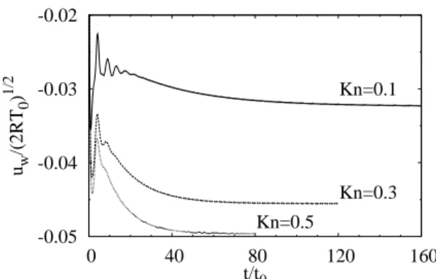
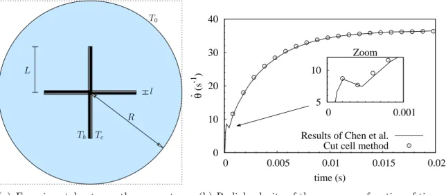
An infinite set of thin plates of height D is located in an infinite channel of width 4D. The distance between two plate centers is 4D. This experiment has been numerically investigated in [42], where the plates are infinitely thin (their thickness is zero). The temperature of the right side of a plate is twice as the temperature of its left side. This induces a force that can be interpreted as the difference between the radiometric force and gas friction, and make the plates move. We point out that all the plates move at the same velocity. After a while, the radiometric force is balanced with gas friction and the total force decreases to zero. At this time, the plates have reached their stationary velocity. In [42] the ES-BGK model is used and simulations are made in a moving reference frame in which the channel velocity is positive while the plates are motionless. The total force applied on the plates is zero for a specific channel velocity which corresponds to the stationary velocity of the plates. In our work, the BGK model is used to described the behavior of the gas and plates are D/10 thick (see Fig. 5(a)). The transient motion of the plates (i.e. plates velocity before the stationary state is reached) can be simulated with the cut cell method in a fixed frame of reference. In that case, the motion depends on the mass of a plate. If we denote by ρ₀ the

initial density of the gas, this mass is set to m = ρ₀D²/2. The computational domain is a rectangle of size 4D×2D that describes the upper part of the channel (Fig. 5(a)). The left and right boundary conditions are periodic so as to simulate the infinite channel. The bottom of the computational domain fits with the center of the channel: specular-reflection boundary condition is applied to take into account the symmetry. At last, the top of the domain corresponds to the wall of the channel, the standard diffuse boundary condition is used. During a whole simulation, there is always one and only one plate in the computational domain: when a plate goes out, an other one comes in. Note that solid and cut cells only appear near this plate. To take its temperature into account, the boundary of the plate is modeled with the diffuse-reflection condition. Finally, the relaxation time and Knudsen number are defined by the relations:

τ = µ

ρRT₀ and Kn = 2

√π

√2RT₀ ρ₀RT₀/µ

. D,

where µis the viscosity of the gas and T₀ the initial temperature of the gas.

Our simulations have been done for a wide range of Knudsen numbers from 10⁻³ to 1.

Converged results are obtained for a velocity grid that contains from 20² to 40² points (this depends on the Knudsen number) and for a spatial mesh made up of 400×200 cells, which means that a plate encloses 10 cells. For coarser grids, the number of cells enclosed in the plate is too small to capture the shape of its edges with enough accuracy. As expected, the magnitude of the velocity of the plates increases until they reach their final velocity, as illustrated for three different Knudsen number on figure 5(b).

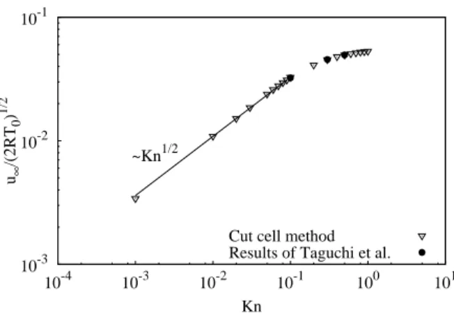
The variation of the stationary velocity of the plates is plotted as function of Kn on figure 6. For small Knudsen numbers, the final velocity seems to be proportional to √

Kn while this velocity tends to a constant for high Knudsen number. These simulations show a good agreement between our results and the results obtained in [42].

4.2 The Crookes radiometer

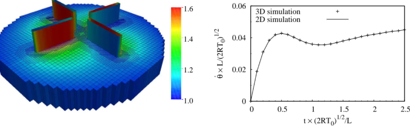
The Crookes radiometer was invented by Crookes in 1874 [12]: it is a glass globe containing four vanes immersed in a low pressure gas. Each vane has one black side and one shiny side, and when the globe is exposed to light, the vanes rotate. This was first understood as a rarefied gas dynamics effect by Reynolds [34], but there are still discussions on the order of magnitudes of the forces involved in this device. We refer to the recent review of Ketsdever et al. [24] for historical details. Recently, numerical simulations improved the understanding of the radiometric effect, like in [41, 42, 37].

The dynamical acceleration process of the vanes has been recently studied in [9]: it uses the unified gas-kinetic scheme combined with a moving mesh approach [10] to simulate the motion of the vanes. In this case, the moving mesh approach is very convenient because the initial mesh just rotates without distortions. In this section, we show that the same results as [9] can be obtained with our cut cell method.