[PENDING] The City as a Complex System. Statistical Physics and Agent-Based Simulations on Urban Models

(1)

HAL Id: tel-00634588

https://tel.archives-ouvertes.fr/tel-00634588

Submitted on 21 Oct 2011

HAL is a multi-disciplinary open access archive for the deposit and dissemination of scientific research documents, whether they are published or not. The documents may come from teaching and research institutions in France or

L’archive ouverte pluridisciplinaire HAL, est destinée au dépôt et à la diffusion de documents scientifiques de niveau recherche, publiés ou non, émanant des établissements d’enseignement et de recherche français ou étrangers, des laboratoires

Agent-Based Simulations on Urban Models

Rémi Lemoy

To cite this version:

Rémi Lemoy. The City as a Complex System. Statistical Physics and Agent-Based Simulations on Urban Models. Economics and Finance. Université Lumière - Lyon II, 2011. English. �tel-00634588�

(2)

Université Lumière Lyon 2

The City as a Complex System

Statistical Physics and Agent-Based Simulations on Urban Models

Thèse pour le Doctorat de Sciences Economiques

Université de Lyon

Laboratoire d’Economie des Transports Institut Rhône-Alpin des Systèmes Complexes

Présentée et soutenue publiquement par

Rémi LEMOY

le 6 octobre 2011

devant la commission d’examen composée de

Directeurs de thèse aaa Pablo JENSEN, Directeur de recherche au CNRS Charles RAUX, Ingénieur de recherche au CNRS

Rapporteurs Marc BARTHELEMY, Chercheur au CEA

André DE PALMA, Professeur à l’ENS de Cachan Examinateurs Jean CAVAILHES, Directeur de recherche à l’INRA

Stéphane DOUADY, Directeur de recherche au CNRS

Florence GOFFETTE-NAGOT, Chargée de recherche au CNRS

(3)

(4)

Acknowledgements

I thank my supervisors Charles Raux and Pablo Jensen who proposed me to carry out this thesis. Their support and guidance during those three years were an essential help.

I also thank all members of the examining committee, and especially Marc Barthélémy and André de Palma.

I am grateful to Eric Bertin for continuing advice and fruitful collaboration. And indebted to Florence Goffette-Nagot, whose help at different times was precious and selfless. I thank also warmly Sébastian Grauwin for stimulating work and conversations during a common PhD experience. My sincere gratitude goes to John Mc Breen for his advice, help and friendship.

I thank Florence Puech for precious advices and a very careful reading of one important chapter. And I am pleased to acknowledge very interesting discussions with Vincent Viguié and also Nicolas Coulombel.

I am grateful to all members of the Transport Economics Laboratory (LET) and of the Rhône-Alpes Complex Systems Institute (IXXI) for making these places pleasant human and scientific environments.

I thank also Serge Latouche, Jacques Testard and Jean-Marc Lévy-Leblond, who allowed me to get in contact with Pablo Jensen during my search for a stimulating thesis project.

I am pleased to thank heartily Jennifer Adam for her love and support.

Finally, I would like to express my gratitude to all the persons who made these three years an enjoyable time, from a scientific and also a human point of view. I hope that they recognize themselves.

(5)

(6)

II Agent-based simulations in urban economics 63

4 An agent-based model of urban economics 65 4.1 Model . . . 67

4.2 Comparison with the analytical results . . . 72

4.3 Emergence of a city . . . 72

4.4 Results of the simulations . . . 74

4.5 Perspectives . . . 82

5 Exploring the polycentric city 85 5.1 Description of the model . . . 86

5.2 Comparison with the analytical model and time evolution . . . 91

5.3 Additions to the standard model . . . 97

5.4 Perspectives and Discussion . . . 106

6 "European" and "North American" cities 111 6.1 Introduction . . . 111

6.2 Evolution with income of housing expenses and value of time . . . 112

6.3 Brueckner et al. [1999] revisited . . . 117

6.4 A logit location choice in the AMM model . . . 120

6.5 Conclusion . . . 127

General conclusion 129 Appendices A Analytical resolution of the AMM model 137 A.1 Resolution of the AMM model . . . 137

(8)

General introduction

The thesis presented here has been carried out at the Transport Economics Laboratory (LET) and at the Rhône-Alpes Complex Systems Institute (IXXI) from 2008 to 2011. This work was co-supervised by Charles Raux, economist, director of LET, and Pablo Jensen, physicist at the Ecole Normale Supérieure (ENS) Lyon. The funding was specifically attributed to a work in urban modeling using agent-based models, so that it is an important part of this work.

The project was designed either for an economist interested in social models inspired from statistical physics, or for a physicist interested in social systems. The author corresponds to the second type, as a physicist by training. So that the point of view presented in this work is strongly influenced by this training in physics. In particular, the first part of this work deals with tools coming from statistical physics and used in the context of social models, while the second part is more closely related to economics.

This work at the border between natural and social sciences raises specific questions thanks to the difference of viewpoints. It can lead to a fruitful exchange of objects and methods.

Such works are also favored by the growing calculation power of computers and the (relative) abundance of available data about socioeconomic systems, which are trends observed in the last years or decades. However, interdisciplinary works also raise some challenges. In addition to the difficulty of communication and the danger of misunderstandings due to different frameworks and even vocabularies, the funding, publication and evaluation of research is still widely disciplinary. Some infrastructures such as IXXI exist to provide exchange possibilities for interdisciplinary work, but they remain somewhat marginal. And teaching is also very disciplinary, which can also raise some problems discouraging such research.

(11)

To cope with the different constraints mentioned, this work focuses on a given object, which is the urban system, but uses different tools in the two main parts of this thesis.

The first part relies more on analytical treatment and presents an approach inspired from statistical physics, while the second one uses agent-based simulations on models which are more closely related to the literature on urban economics.

Before presenting more in detail the content of this thesis, and after the description of the scientific inter-disciplinary context, let us give some elements of socioeconomic context.

What is at stake in the study of urban systems, linking land use and transport? What are the challenges which cities are facing or will be facing in the next years or decades? We give here a broad overview of the issues which are linked more or less directly to urban systems, and in particular to housing and transport in urban areas.

The context is global, at a world scale, even if very different situations can be encountered in particular cases. Indeed, it is now for instance consensual among scientists that the global climate is changing (America’s Climate Choices: Panel on Advancing the Science of Climate Change [2010], Oreskes [2004]). More precisely, the average temperature on earth is increasing, hence this climate change is also named global warming. The average global temperature has increased during the 20th century of approximately 0.7^◦C (Intergovernmental Panel on Climate Change [2007]), which is very significative. But the effects in particular locations may differ greatly, as the global climate is a perfect example of very complex system.

Nonetheless, there is also a scientific consensus on the fact that greenhouse gases emissions due to human activities, and for instance transport and housing, which will be studied in this work, represent an important if not essential contribution to the global warming (see the same sources).

A second big challenge which humanity is facing or will be in a near future is linked to the decreasing reserves of fossil fuels such as oil and coal (International Energy Agency [2010]) and their subsequent increasing price. Peak oil is especially worrying, as oil is used as a fundamental raw material in many different contexts, not only as fuel. Its increasing price led already to begin the extraction of unconventional oil in spite of its lesser efficiency and greater environmental impact. Biofuels, also less efficient, are becoming a viable source of fuel because of the increasing price of oil. Their growing production is associated with different issues, for instance the "food vs. fuel" debate, as biofuels may be one of the causes of the 2008 food crisis, which caused food riots in a number of countries.

Associated with the decreasing reserves of fossil fuels are the decreasing reserves of many

(12)

General introduction

metals (Gordon et al. [2006]), which are important components of many modern devices, for instance those which produce renewable energy like solar panels (Bihouix and de Guillebon [2010]), but also electric cars (or more generally most electric or electronic devices). This complicates the problem even more.

Warnings against these decreasing reserves of fossil fuels and metals reach as far back as Meadows and Club of Rome [1972], Georgescu-Roegen [1986] (these sources providing interesting attempts to promote a science of complex systems, by linking statistical physics and economics for the second one). But almost no political measures have been taken for the moment.

More political consensus can be found on the reduction of greenhouse gases emissions.

France for instance pledged to reduce its emissions by a factor of 4 in 2050 compared to 1990.

But 2050 seems very far away from a human and political point of view. Internationally, many such commitments have been taken by states and communities.

In France, among other countries, the main response to the increasing price of energy associated to these challenges is the use of nuclear power plants. However, more and more concern is raised by the use of nuclear energy, following the Fukushima Daiichi nuclear disaster, which began in March 2011, and recalled other nuclear accidents, which relatively spared France for the moment. As the question of security is asked anew (several European countries decided recently to abandon progressively the use of nuclear energy), the other problems and constraints of this energy source are also discussed. For instance, the fact that there is no viable solution in sight for nuclear waste, the difficulty to deal with peak hours of electricity consumption and the close link between civil and military use of nuclear power. Nuclear fusion, which produces less toxic waste, will not be a possible energy source in the next years or decades, as it is still at a fundamental research stage for the moment, in spite of massive investments.

In this context of increasing price of energy linked to decreasing reserves of different materials, and of climate change linked to human emissions of greenhouse gases, cities can be seen as focal points. Cities consume over 60% of the global energy production and contribute to 70% of the world’s emissions of greenhouse gases. More than half of the world population now lives in cities, and this share is expected to grow to reach 70% by 2050 (United Nations [2008]). Furthermore, inequalities of access to resources are very high between and among countries (Milanovic [2005]). Cities in particular are places where the richest and the poorest coexist. This creates social tensions which are yet another challenge.

(13)

The sector of transport produces 20% of total greenhouse gases emissions related to human activities in Europe, and 30% in the USA (OECD [2008]). Housing is also a major sector of emissions. As a consequence, studying the interaction between housing and transport in cities is at the heart of the problems evoked previously. In addition, cities are particularly interesting places to develop environmental friendly transportation, due to the many opportu- nities available on short distances. Bike use for instance can be very practical in urban areas.

However, cities such as Copenhagen or Amsterdam with bicycles accounting for around 30%

of all transportation are exceptions in Europe and in the world.

Of course, urban models such as those presented in this thesis are not proposing the solutions to really deal with the challenges we evoked. The main challenge is actually a question of social and political consciousness and will. But all these challenges provide a framework for urban modeling. Hence, the central question regards the "sustainable" city: if the models manage to grasp even roughly the socioeconomic reality of urban systems, or at least to help conceiving their complexity, which urban forms would consume less energy for transport and housing? And what are their consequences on the welfare of different social groups and on social inequalities? More generally, what are the main determinants of city structure, and which factors can explain the differences encountered worldwide?

These questionings constitute the socioeconomic context of this thesis. The scientific context was evoked earlier through the inter-disciplinary collaboration between physicists and economists. One more element should be added regarding the scientific context in economics.

Although computer simulations are widely used in physics to make up for analytical treatment when it is limited, the use of simulations is still marginal in economics, and seems to be seen as very unsatisfactory. Hence, an important aim of the part of this thesis which is oriented towards economics is to show that computer simulations, and in particular agent-based models in this work, can provide an interesting complement to analytical resolution.

As stated previously, this work is divided in two main parts. The first part concerns the three first chapters of this thesis, and corresponds to a physicist’s point of view on simple socioeconomic models. The second part consists in the three last chapters and deals with agent-based models closely related to the standard urban economics model (Alonso [1964], Muth [1969], Mills [1967], see also Fujita [1989]).

(14)

Resolution of a Schelling-like segregation model

The first chapter presents a statistical physics framework which enables us to solve analytically a Schelling-like model. Schelling’s model (Schelling [1971]) is a famous toy model dealing with spatial segregation. It can be seen as one of the first agent-based models, as Thomas Schelling studied it even before computer simulations were used in social sciences.

The main ingredient of our resolution is the introduction of a state function, which reflects individual preferences and dynamics of socioeconomic models. In this framework, standard statistical physics tools can be used on simple models coming from social sciences, in a method- ological approach which can be linked to potential games (Monderer and Shapley [1996]). The decision to move is taken as a logit rule, which is a standard choice in social models (Anderson et al. [1992]).

Schelling’s model gives a counter-intuitive result on the link between "microscopic" behavior of social or economic agents, and the "macroscopic" outcome in the whole system studied.

The description of agents’ behavior is very simple. Agents make location choices depending on the composition of their neighborhood. These choices are to optimize a welfare function called utility function. For a given agent, this function is in this work a peaked function of the number of agents similar to himself in the neighborhood. Although agents desire a mixed environment, a small asymmetry in the utility function, results in segregated macroscopic patterns. This is a surprising result, as it is quite counter-intuitive to predict such a global equilibrium state of the system when knowing agents’ rules of behavior.

We use this model to study the difference between individual and collective dynamics of agents. To this end, we introduce a continuous parameter leading the model to shift contin- uously from "individualistic" dynamics, where agents care only about their personal welfare, to "collective" dynamics, where the global welfare is the objective. These rules of behavior illustrate an important difference between social sciences models (individual dynamics) and systems usually studied by statistical physics (collective dynamics). The main achievement of this work is to introduce a potential function linking both.

Utility and chemical potential

In the second chapter, this study is brought closer to urban economics modeling. Indeed, we use this statistical physics framework in a different context, where space is not homogeneous, contrary to Schelling’s model. The dynamics is still given by a logit rule with a parameter that

(15)

can be seen as a temperature from a physicist’s point of view. In economics, this parameter is interpreted as the width of a distribution of tastes. In this model with non-homogeneous space, we are led to introduce a chemical potential in our social model, as a Lagrange multiplier accounting for the conservation of agents, instead of particles, as is the usual case in statistical physics. When the temperature is not zero, the utility (welfare of agents) is not homogeneous in the whole system at equilibrium, contrary to standard results for socioeconomic models.

However, the chemical potential we introduce, which adds an entropic contribution to the utility term, is homogeneous across the system. To illustrate this framework, we study a model corresponding to a simplified version of the standard urban economics model. The essential simplifying hypothesis consists in supposing that price and density are directly related. As a consequence, the statistical physics framework presented in the first chapter can be used.

A numerical resolution of this simple model allows us to link these results to the economic literature on the introduction of a heterogeneity of tastes in the standard urban economics model (De Palma and Papageorgiou [1988], Anas [1990]).

An important condition of the model making analytical resolution possible is that the dynamics respects detailed balance (see Van Kampen [1992], Evans and Hanney [2005]).

Some conditions are derived to ensure that it is the case in the model we study. However, we perform agent-based simulations on a model which does not respect these conditions, that is, outside the domain of validity of our statistical physics framework. We observe that our result concerning the homogeneity of the chemical potential can be valid in other cases.

A probabilistic model of housing price formation

The third chapter builds on a hypothesis of the second one, which postulates in the simple model studied a direct relationship between density of inhabitants and price at a given location. We design a simple model of urban housing market which, through the use of an ergodic hypothesis, links the time variations of the price of a representative flat to the spatial variations of price within a virtual city. Price evolves as a function of the occupancy of the flat: it increases when the flat is occupied (highly demanded), and decreases if the flat is empty. Agents moving into or out of this flat will determine the evolution of its price. This is a schematic way to represent urban price dynamics and link it to the density of inhabitants.

However, this work in progress raises a question regarding the relationship between two definitions of the density, one linked to time variations and corresponding to the mean oc-

(16)

cupancy in time of the flat, and the other being a "spatial" constraint in the virtual city.

Indeed, the ergodic hypothesis allows us to link the mean occupancy in time of a given flat to the spatial variation of price in the virtual city. But the simulations show that these two quantities do not coincide, a phenomenon which deserves further investigation.

Still, these simulations show that the model reaches an equilibrium state which is indepen- dent of the initial conditions. The evolution of this equilibrium as a function of the different parameters of the model is a perspective of work. The influence on price distributions of the density of agents, which is the most "physical" parameter of the model, is studied in this chapter. An interesting perspective is linked to the simplicity of the dynamics used. It should make an analytical resolution of the model possible in some limiting cases.

An agent-based model of urban economics

The second part of this work relies less on analytical results, in order to study more descrip- tive models. This research is directly linked to the urban economics literature, but the use of simulations corresponds more to a physicist’s approach. This work is inspired for instance by Caruso et al. [2007], Brueckner et al. [1999]. Chapter 4 presents an agent-based model using simple and intuitive dynamics. From a random initial state, a urban system is led by the dynamics to an equilibrium corresponding to a discrete version of Alonso’s model (Alonso [1964]). This standard urban economics model presents an analytical, static residential equilibrium of agents in a urban area. The dynamics of the agent-based model are directly inspired by the competition for land of the analytical model, where the highest bidder wins.

We find a good agreement between the results of the analytical and agent-based models.

Then, building on this agreement, the agent-based model is used to study phenomena which are less tractable analytically. In particular, this chapter, following Brueckner et al. [1999]

or Wu and Plantinga [2003], considers the introduction of a positive amenity in the urban system. The agent-based simulations enable us to study the influence of this amenity on the city. Different variables indicate the behavior of the urban model. The utility of agents is associated to their economic welfare. When two income groups are introduced, the evolution of the gap in welfare between both income groups can be studied when some parameters are changed. The commuting distances of agents are also an important indicator of the urban system.

Different urban social structures can be observed in North American and European cities.

(17)

North American cities tend to have rich households in the periphery and poorer ones near the center, while European cities tend to present an inverse configuration, as described by Brueckner et al. [1999]. Attempts are made using the agent-based model to have these social structures emerge from the interactions between agents. But the results seem unsatisfactory.

Indeed, the standard urban economics model results usually in a "North American" configuration, with rich agents in the periphery. The "European" city is more difficult to obtain within this model.

The introduction of a travel time cost alone does not induce the "European" configuration, if realistic values of this time cost for rich and poor agents are studied. And the use of a log- linear utility function leads us to define a higher preference of rich agents for the amenity introduced in this chapter, in order to obtain the "European" city configuration. Although this can be sufficient to have this result, the ingredient is exogenous and disturbing from a modeling point of view. The equilibrium obtained is shown to be very sensitive to a difference of location between the work center and the amenity center, in a two-dimensional city.

Exploring the polycentric city

Chapter 5 uses a version of the agent-based model introduced in chapter 4, where the dynamics is simplified, but leads still the model to its equilibrium. The goal of this chapter is to deal with the question of the polycentric city. It is indeed an issue in the economic literature, to determine if a city with several employment centers is more desirable from a point of view of sustainability than a monocentric city. And the polycentric framework seems also closer to the empirical reality of urban systems.

A detailed discussion is given on the existence and uniqueness of the equilibrium of the different models studied. The existence is proved in Fujita and Smith [1987], and uniqueness is proved in Fujita [1985] in a certain monocentric framework. A mapping between mono- and polycentric models allows us to extend this result to some polycentric models we study.

And qualitative arguments are used in the other cases.

A comparison is realized between the results of the standard analytical monocentric model with two income groups and those of the agent-based model. The analytical model is solved numerically thanks to a dedicated procedure (see Fujita [1989]). The agreement between analytical results and agent-based simulations is very good. The chapter details the conditions guaranteeing that the agent-based model reaches a discrete version of the analytical

(18)

equilibrium. We insist on the close link between the analytical results and the agent-based simulations because the latter have still to prove their value in the economic literature, which valuates analytical results more.

The study of the polycentric city in itself is then presented, with different polycentric models where agents have different constraints, and represent single workers in some models and two-workers households in another, with some households composed of two persons working in different employment centers. As in chapter 4, the evolution of certain global variables conveys the economic, environmental and social outcomes of these models.

Polycentrism is globally seen as desirable in these models, as it favors the welfare of agents and tends to decrease commuting distances. But a negative effect in terms of greenhouse gases emissions is the fact that it increases housing surfaces, and thus heating and cooling needs.

As a consequence, calibrated urban models are needed to really assess the environmental outcome of such models. A first attempt to calibrate Muth’s model, which includes building construction (Muth [1969]) on the Grand Lyon urban area is presented in appendix B.

"European" and "North American" city

In chapter 6, the model presented in chapter 5 is applied to different utility functions, in order to come back to the question of "European" and "North American" cities addressed in chapter 4. Indeed, chapters 4 and 5 use a Cobb-Douglas utility function, which is the most used utility function because of its handy character for analytical resolution. But of course, the form of the utility function determines the results of the model, and other expressions are studied in this chapter 6.

More precisely, taking into account the evolution with income of the value of time of agents and of the budget share of housing yields in the most standard version of Alonso’s model (using a Cobb-Douglas utility function) "European" city patterns. A characteristic distance is defined, at which the locational behavior of income groups changes. This allows us to model the emergence of a rich periurban area in "European" cities.

The hypothesis of Brueckner et al. [1999] concerning a central amenity in European cities is then revisited. Indeed, a utility function making rich agents valuate the amenity more than poorer ones can result in a "European" pattern. This result is reproduced with our agent- based model. This work shows in addition that richer social patterns can emerge than just wealthy agents in the center and poorer ones in the periphery (or vice versa), in agreement

(19)

with the first part of the chapter.

Finally, a logit location choice is introduced in the agent-based model, as a means to lessen the dependence of the results of the model on the choice of the utility function. In fact, including a logit model introduces randomness in the location choice, and blurs the patterns dictated by the utility function. This study bridges the gap with the first part of this thesis, as this last model is also shown to verify the main result obtained in chapter 2. The chemical potential is homogeneous at equilibrium in the agent-based model, which is surprising as this model seems very far from fitting in the domain of validity of the statistical physics framework of chapter 2. More work is needed to link this result with the economic literature, especially De Palma and Papageorgiou [1988] and Anas [1990].

(20)

Part I

Statistical physics and urban models

(21)

(22)

Chapter 1

Solution of a Schelling-like segregation model

1.1 Introduction

This chapter presents the contribution of this author to a collective work (Grauwin et al.

[2009]). The model we study is a simplified version of the segregation model of Thomas Schelling (Schelling [1971]). The original model is not solvable analytically, so that some simplifications are made here to allow an analytical resolution. The important point is that under these simplifications, the main phenomenon of Schelling’s model, a non-intuitive segregation emerging whereas agents are looking for integration, is conserved. We also explore how this

"fated" segregation can be broken by introducing a more altruistic behavior of agents, inspired from usual dynamics in physics. This allows us to deal with the question of individual and collective dynamics, which seems to be one important difference between social systems and systems usually studied by statistical physics.

The main idea of this work is detailed in Grauwin et al. [2009]. A function, which is called

"link function" in the article, is introduced to describe the dynamics of the model like the dynamics of usual statistical physics models. This can be linked to the literature on potential games (Monderer and Shapley [1996]). From a physicist’s point of view, this function can be thought of as an effective Hamiltonian. It allows in the context of this simplified Schelling model to bridge the gap between social sciences and statistical physics. Namely, economic or social agents move in social models to maximize their utility (Mas-Colell et al. [1995]), an individual function which describes their welfare with respect to the variables studied by the

(23)

model. In statistical physics, particles move to minimize the (free) energy (Goodstein [1985]), which is a global function of the system. This can be interpreted intuitively by observing that physical particles have no individuality, compared with social agents. But this characteristic makes the modeling of their behavior easier. The introduction of this link function allows the use of a statistical physics formalism to solve the problem by finding the equilibrium state.

1.2 Description of the model

This segregation model describes the location choices of agents in a city and how segregation can emerge at a macroscopic level from interactions between agents at a microscopic level. The model is very simple and schematic: two groups of agents are studied, which are distinguished by their "colors", red and green for instance. These agents live on a two-dimensional grid, where each cell can accommodate one agent only, and some cells are left vacant. Agents move to maximize their welfare, which depends only on the number of agents in their neighborhood who have the same color as themselves.

Instead of using interactions with nearest neighbors, for instance Moore neighborhoods, agents are located in quarters and interact only within a quarter, which is an important difference with the standard Schelling model.

Let us first give a brief description of the notations used to characterize this social system.

1.2.1 Notations

The simulation space is a two-dimensional grid, composed ofQblocks labeled by q= 1, ..., Q.

Each block is in turn composed of H cells. Two groups of agents, described as red and green, live on this space, each agent occupying one cell. There are overall N_r red and N_g green agents, with N_r +N_g < QH, the rest of the cells remaining vacant. This is illustrated on figure 1.6.

A microscopic configurationxof the system is given by the knowledge of the state of each cell: red, green or empty. A coarse-grained configuration corresponds to the knowledge of the numbers of red and green agents in each block, described respectively by n_qr and n_qg. The utility function of a red (respectively green) agent is written u_R(n_qr/H) (respectively u_G(n_qg/H)). It depends only on the number of agents of the same kind in the block where the considered agent lives. Agents move in order to maximize this utility function.

(24)

1.2. Description of the model

The link function, which allows to describe the individual dynamics by a global quantity, is denotedL(x). This global function must reflect each individual move, which can be written

∆u= ∆L: for any move, the variation of the (individual) utility of the moving agent is equal to the corresponding variation of the link functionL, which is a global function.Then the link function corresponds, in each block, to the sum of agents’ utility as they are introduced one by one in the block:

L(x) = X

q

nqr

X

m=0

u(m/H) +

nqg

X

m=0

u(m/H)

To study the link between individual and collective dynamics, the total utilityU is introduced. It is given in a configuration x by the sum of all individual utility functions:

U(x) =X

q

(nqru(nqr/H) +nqgu(nqg/H))

An interesting question can be raised: the difference between collective and individual dynamics. A simple way to study it is to introduce a continuous parameter α, 0≤α ≤1, which will determine what determines the dynamics of the system: the function driving the system is a cost function denoted by C, and its expression is chosen as C(x) = (1−α)L(x) +αU(x).

For α = 0, individual decisions only are taken into account in the dynamics, and for α = 1, only the global utility matters.

1.2.2 Dynamics

The evolution of the system is simple. Consider an agent and a vacant cell in the city. Let

∆u be the variation of utility the considered agent would experience when moving to the candidate cell and ∆U the corresponding variation of the global utility. Then each agent has a probability W(x → y) per unit time to move in a given vacant cell, given by a logit rule (Anderson et al. [1992])

W(x→y) = 1

1 +e^−∆C/T = 1

1 +e−(C(y)−C(x))/T

where x and y are the states of the system before and after the move, and

∆C = (1−α)∆u+α∆U = ∆u+α(∆U−∆u)

(25)

is the variation of the global cost function associated to the considered move. Depending on the value of the "altruism" parameter αbetween 0 and 1, the agent will move based more on his individual utility gain or rather on the variation of the global utility of the system.

1.2.3 Stationary probability distribution

This system obeys a master equation given by

∂P(x, t)

∂t =X

y6=x

P(y, t)W(y→x)−P(x, t)W(x→y)

where P(x, t) is the probability that the system is in state x at timet.

Let us now introduce the probability density P_s(x)given by P_s(x) = exp(C(x)/T)

P

zexp(C(z)/T)

It can be verified that for all couples of statesxandythis probability density satisfies detailed balance:

P_s(x)W(x→y) = exp(C(x)/T) P

zexp(C(z)/T) × 1

1 + exp[−(C(y)− C(x))/T]

= exp(C(y)/T) P

zexp(C(z)/T) × exp(C(x)/T)

exp(C(y)/T) + exp(C(x)/T)

= P_s(y)W(y→x)

Then Ps(x) is the equilibrium probability density, which describes the probability of each microscopic state x at the equilibrium of the model. Let us now study the coarse-grained description of this system and its equilibrium.

1.2.4 Coarse-grained description

Instead of describing the system by the knowledge of the state of each cell, we describe it now by the knowledge of the numbers of red and green agents in each block, n_qr and n_qg. We denote this coarse-grained state by {(n_qr, n_qg)}. There are _n ^H!

r!ng!(H−nr−ng)! ways of ordering n_r undifferentiated red agents and n_g undifferentiated green agents in H cells. Indeed, there

(26)

1.2. Description of the model

are _(n ^H!

r+ng)!(H−nr−ng)! ways of placing the vacant cells and ⁽ⁿ_n^r⁺ⁿ^g^)!

r!ng! ways of placing the agents’

colors. So that the stationary probability of a coarse-grained state{(n_qr, n_qg)}can be written:

Π({(nqr, nqg)}) = 1 Z

Y

q

H!

n_qr!n_qg!(H−n_qr−n_qg)!e^C({(n^qr^,n^qg^)})/T

= 1 Z exp

H/T X

q

f(n_qr, n_qg, T, H)

where Z is a normalization constant, and f(n_qr, n_qg, T, H) = −T

H lnnqr!nqg!(H−nqr−nqg)!

H!

+ αn_qr H ur

n_qr H

+αn_qg H ug

n_qg H

+ (1−α)1 H

nqr

X

m=0

u_rm H

+ (1−α)1 H

nqg

X

m=0

u_gm H

with u_r and u_g the utility functions of red and green agents, depending only on the number of agents of the same color in the block. The configurations that maximize the potential F(x) = P

qf(n_qr, n_qg, T) are the more probable to come up. In the limit H/T → ∞, these configurations are even the only ones that will appear in the stationary states (since Π(x)/Π(y) = e^H/T^(F^(x)−F(y)) →0for F(x)−F(y)<0and H/T → ∞).

1.2.5 Continuous limit

In the limit H → ∞, by keeping constant the mean density ρ0 = N0/H and the density of each block ρq =nq/H (ρq hence becoming a continuous variable), one has thanks to Stirling’s formula:

ln

n_r!n_g!(H−n_r−n_g)!

H!

' H h

ρqrlnρqr+ρqglnρqg

+(1−ρ_qr−ρ_qg) ln(1−ρ_qr−ρ_qg)i

(27)

and the stationary distribution can be written as:

Π({(ρ_qr, ρ_qg)}) = 1 Z

Y

q

e^{H/T f}^(ρ^qr^,ρ^qg^,T⁾

where the "block-potential" f is

f(ρ_r, ρ_g, T) = −T ρ_rlnρ_r−T ρ_glnρ_g −T(1−ρ_r−ρ_g) ln(1−ρ_r−ρ_g) + αρ_ru_r(ρ_r) +αρ_gu_g(ρ_g)

+ (1−α) Z ρr

0

ur(ρ⁰)dρ⁰+ (1−α) Z ρg

0

ug(ρ⁰)dρ⁰

The problem hence results in finding the set {(ρ_qr, ρ_qg)} which maximizes the potential F =P

qf(ρ_qr, ρ_qg, T) with the constraints P

qρ_qr =Qρ_0r and P

qρ_qg =Qρ_0g, whereρ_0r and ρ_0g are the global densities of red and green agents.

When comparing this result with the result of the one color model detailed in Grauwin et al. [2009], it can be remarked that for a zero temperature the two colors model described here is obtained by summing two one color models, one for each color. But at a non-zero temperature the −T(1−ρr−ρg) ln(1−ρr−ρg) term links both groups of agents.

1.3 Phase transitions

The simplest result of the model corresponds to having a homogeneous phase ρ = (ρ_r, ρ_g) in the whole city. But this homogeneous phase may be unstable with respect to phase separation.

Let us split the system into two phases of densitiesρ₁ = (ρ_1r, ρ_1g)andρ₂ = (ρ_2r, ρ_2g). The constraint that the overall densities of particles/agents are ρ₀ = (ρ_0r, ρ_0g)is expressed by the lever rule:

( Q₁+Q₂ =Q Q₁ρ₁+Q₂ρ₂ =Qρ₀

whereQ₁ andQ₂ are respectively the number of blocks of densityρ₁ andρ₂. The homogeneous phase is stable against phase separation if for all ρ₁ and ρ₂

Q₁f(ρ₁) +Q₂f(ρ₂)< Qf(ρ₀) (1.1)

(28)

1.4. With a peaked utility function

Geometrically, this inequality corresponds to requiring that f(ρ) is a concave function.

When the concavity requirement is violated, phase separation will occur for certain values of ρ₀. The equilibrium densities ρ₁ and ρ₂ are such that the line that joins the points (ρ₁, f(ρ₁)) and (ρ₂,f(ρ₂)) is part of the concave hull of the function.

In the two colors model there is also a possibility that the system is split into 3 phases of densities ρ₁ = (ρ_1r, ρ_1g), ρ₂ = (ρ_2r, ρ_2g) and ρ₃ = (ρ_3r, ρ_3g), which is absent in the sim- pler model presented in Grauwin et al. [2009]. The constraint that the overall densities of particles/agents are ρ₀ = (ρ_0r, ρ_0g) is in the 3 phases case:







Q₁ +Q₂+Q₃ =Q Q₁ρ_1r+Q₂ρ_2r+Q₃ρ_3r =Qρ_0r Q1ρ1g+Q2ρ2g+Q3ρ3g =Qρ0g

where Q₁, Q₂ and Q₃ are respectively the number of blocks of density ρ₁,ρ₂ and ρ₃.

And the equilibrium densities ρ₁, ρ₂ and ρ₃ are now such that the plane that joins the points (ρ₁, f(ρ₁)), (ρ₂,f(ρ₂)) and (ρ₃,f(ρ₃)) is part of the concave hull of the function. For some values of the parameters there may even be 4 points of the same plane belonging to the f function and its concave hull. In this case there will be a continuum of possible values of Q1, Q2, Q3 and Q4 verifying the global density constraints.

1.4 With a peaked utility function

1.4.1 Expression of the f function

Let us consider for both color groups the asymmetrically peaked utility function (Pancs and Vriend [2007]) u_r=u_g =u defined for m <1 as:

u(ρ) = 2ρ if ρ≤0.5 u(ρ) = m+ 2(1−m)(1−ρ) if ρ >0.5

This function is presented on figure 1.1. Agents have a real taste for integration, as they are most satisfied when only half of their environment consists in agents of the same color as them. But they prefer total segregation, providing them with a utility m, which is usually supposed to be non-negative, to being "alone among strangers" (or vacant cells), which gives

(29)

a zero utility.

Figure 1.1: Asymmetrically peaked utility function, with m= 0.5.

Then forρ_r ≤0.5and ρ_g ≤0.5, the f function is given by:

f(r, g) = −T rlnr−glng−(1−r−g) ln(1−r−g)

+ (1 +α)(r² +g²)

∂f

∂r(r, g) = −T lnr−ln(1−r−g)

+ 2(1 +α)r

∂²f

∂r²(r, g) = −T /r−T /(1−r) + 2(1 +α)

(Partial derivatives relative to g are obtained by replacing g ↔r) Forρ_r >0.5 and ρ_g ≤0.5,

f(r, g) = −T rlnr+glng+ (1−r−g) ln(1−r−g)

−(1 +α)(1−m)r² + (2−m)r−(1−α)(2−m)/4 + (1 +α)g²

∂f

∂r(r, g) = −T lnr−ln(1−r−g)

−2(1 +α)(1−m)r−(2−m)

∂²f

∂r²(r, g) = −T /r−T /(1−r−g)−2(1 +α)(1−m)

∂f

∂g(r, g) = −T lng−ln(1−r−g)

+ 2(1 +α)r

∂²f

∂r²(r, g) = −T /g−T /(1−r−g) + 2(1 +α)

The situation ρ_r ≤0.5 and ρ_g >0.5 can be obtained by replacing g ↔r in the previous

(30)

paragraph.

1.4.2 At zero temperature

f is concave in ρ_r and ρ_g for ρ_r and ρ_g ≤0.5. Forρ_r >0.5 and ρ_g ≤0.5, f is concave in ρ_r and convex in ρg (and conversely for ρr ≤0.5 and ρg >0.5, f is concave in ρg and convex in ρr).

The concave hull of the function has a different form for different values of the parameters α and m:

• for α ≥ _3−2m¹ the points 0,¹₂, f(0,¹₂)

and ¹₂,0, f(¹₂,0)

belong to the concave hull whereas forα≤ _3−2m¹ they are replaced by the points 0,ρ˜2, f(0,ρ˜2)

and ρ˜2,0, f( ˜ρ2,0) with ρ˜₂(α, m) = ¹₂q

1−α 1+α

2−m

1−m (see the resolution of the model with agents of only one color in Grauwin et al. [2009]).

• for α≥ _4−3m^m the point ¹₂,¹₂, f(¹₂,¹₂)

belongs to the concave hull whereas forα < _4−3m^m it does not.

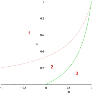
So there are three possible situations, shown on figure 1.2:

Figure 1.2: The domains of different concave hulls for different values of m and α

(31)

• α ≥ _3−2m¹ (which will be case 1)

• _4−3m^m ≤α≤ _3−2m¹ (case 2)

• α < _4−3m^m (case 3) Case 1

The number and composition of the phases depend on the global densities ρ₀ = (ρ_0r, ρ_0g)(see figure 1.3). In part A of figure 1.3, the system separates into 3 or 4 phases of densities (0,0),

Figure 1.3: Domains of different phases for different global densitiesρ₀ = (ρ_0r, ρ_0g)in case 1

(0,¹₂),(¹₂,0)and (¹₂,¹₂) in respective quantities Q₁, Q₂,Q₃ and Q₄, which must verify







Q2+Q4 = 2Qρ0g

Q3+Q4 = 2Qρ0r

Q₁+Q₂+Q₃+Q₄ =Q

The system can build either 3 or 4 phases because red and green agents do not "see" each other: their utility is maximal when half of the block is filled with agents of their color, the other half being either empty or filled with agents of the other color. A simulation of a (discrete) stationary configuration corresponding to this case is shown as illustration on the left panel of figure 1.6.

(32)

In part B, the system separates into 2 phases of densities (^ρ_1−2ρ^0r^−ρ^0g

0g ,0) and (¹₂,¹₂) with respective weights Q₁ = Q(1−2ρ_0g) and Q₂ = 2Qρ_0g. And symmetrically in part C the system separates into 2 phases of densities (0,^ρ_1−2ρ^0g^−ρ^0r

0r ) and (¹₂,¹₂) with respective weights Q₁ =Q(1−2ρ_0r)and Q₂ = 2Qρ_0r.

Case 2

The number and composition of the phases depend again on the global densities as shown on figure 1.4. In part A of figure 1.4, the system separates into 3 phases of densities (0,0),

Figure 1.4: Domains of different phases in case 2

(0,ρ˜₂(α, m)) and ( ˜ρ₂(α, m),0) in respective quantities Q₁ = Q(1− ^ρ^0r_ρ^+ρ_˜ ^0g

2 ), Q₂ = Q^ρ_ρ^0g_˜

2 and

Q₃ =Q^ρ_ρ^0r_˜

2 .

In part B the system is split into 3 phases of densities (0,ρ˜2), ( ˜ρ2,0) and (¹₂,¹₂)in respective quantities Q1 =Q^ρ^˜²^(2ρ^0g_{2 ˜}_ρ^−1)+ρ^0r^−ρ^0g

2( ˜ρ2−1) ,Q2 =Q^ρ^˜²^(2ρ^0r_{2 ˜}_ρ^−1)+ρ^0g^−ρ^0r

2( ˜ρ2−1) and Q3 =Q^ρ^˜²^−ρ_ρ_˜^0r^−ρ^0g

2−1 .

In part C the phase decomposition is the same as in part B of case 1 and in part D it is the same as in part C of case 1.

Case 3

The different domains of phase decomposition are shown on figure 1.5. In part A of figure 1.5 the system separates into 3 phases like in part A of case 2.

(33)

Figure 1.5: Domains of different phases in case 3

In part B there are 2 phases of densities(ρ_0r+ρ_0g,0)and (0, ρ_0r+ρ_0g)in respective quantities Q₁ =Q_ρ ^ρ^0r

0r+ρ0g and Q₂ =Q_ρ ^ρ^0g

0r+ρ0g. A (discrete) stationary configuration corresponding to this case is given on the left panel of figure 1.6.

1.4.3 Interpretation

At zero temperature, this two colors model is indeed very similar to the one color model presented in Grauwin et al. [2009]: both groups of agents see each other only as occupied cells (the utility of a red agent does not depend on the number of green agents in the block).

The only difference with two superimposed one color models lies in the fact that blocks with density (¹₂,¹₂) are full of agents with maximal utility and cannot take in more agents, so that for certain values of the global densities, in cases 1 and 2, there is a phase of half-red, half-green blocks and another phase containing the excess of the more numerous type of agents with a higher density (and thus an inferior utility). An illustration of equilibrium configurations is given on figure 1.6. Grauwin et al. [2009] provide an illustration of these same equilibrium configurations with continuous neighborhoods, to illustrate the similar behavior of this model with block neighborhoods and of the standard Schelling model.

(34)

1.5. Conclusion

Figure 1.6: Stationary configurations of the city with equal numbers of red and green agents, 10% of the total number of cells being vacant, andm = 0.5. On the left panel, α= 0, which illustrates case 3, part B: complete segregation with an "individualistic" behavior of agents.

On the right panel, α = 1, which illustrates case 1, part A: more integrated pattern with an

"altruistic" behavior of agents.

1.4.4 For non-zero temperatures

At very high temperatures, the entropic term of the f function is the leading term, and as it is a concave one, the function is concave everywhere : for any density ρ0 = (ρ0r, ρ0g), the system stays in an homogeneous phase because of the strong noise.

For intermediary values of the temperature, the system has a behavior which is intermediary between a noise driven one and the one it has at zero temperature. A numerical resolution such as the one performed in the next chapter on a different model is needed to find the equilibrium configuration of the system, but it is beyond the scope of this work.

1.5 Conclusion

The introduction of a potential function linking individual preferences to the global dynamics of the social system we study allows us to solve analytically a simplified version of Schelling’s segregation model. In addition, the simplification we introduce, that is, keeping neighborhoods fixed to have local interactions in a determined environment, conserves the qualitative behavior of the original model. This work can be seen as a first example of simple solvable social models which can be studied with equilibrium statistical physics tools. The method,

(35)

which consists in introducing a global potential function representing individual dynamics, could be used on other social models. In the next chapter, we show how it can be applied to a model with a non homogeneous space, polarized by a punctual employment center.

(36)

Chapter 2

Socio-economic utility and chemical potential

This chapter presents a work which has been carried out in collaboration with Eric Bertin and Pablo Jensen. It is published as Lemoy et al. [2011a].

Socio-economic sciences and statistical physics are both interested in the evolution of systems characterized by a large number of interacting entities. These entities can for instance be economic or social agents in social sciences (Smith [1784], Schelling [1971], Latour [2005]), atoms or molecules in statistical physics (Cotterill [2008], Goodstein [1985], Balescu [1975]).

The question of the emergence of macroscopic patterns from the interactions of a large number of microscopic agents is studied by both fields of science. In statistical physics, a quantitative framework has been developed over the last century, allowing the equilibrium behaviour of large assemblies of atoms or molecules to be handled precisely (Balescu [1975]).

In socio-economic models, the preferences of individuals are usually characterized by a utility function, which describes their welfare with respect to their current situation or environment. Each individual or agent wants to maximize his own welfare. Decisions (e.g., moving to a more convenient place) are thus taken in a purely selfish way, while in physics the motion of particles is governed by the variation of the total energy. Recently, a global function linking individual decisions to the variation of a global quantity has been introduced to describe some classes of socio-economic models (see Grauwin et al. [2009], Goffette-Nagot et al. [2009]). This approach then allows such models to be described with statistical physics

(37)

tools. Importantly, the equilibrium state can then be calculated by maximizing a state function (akin to a free energy) instead of having to solve a complicated Nash equilibrium of strategically interacting agents.

The question we investigate in this chapter is whether this physical description of socioeconomic models can be extended to other basic concepts of statistical physics, such as the equalization of thermodynamic parameters like temperature or chemical potential. The equalization of these quantities throughout the system precisely results from the conservation of the conjugated extensive quantities, namely the energy or the number of particles. Although there is no notion of energy in socio-economic models, the dynamics indeed conserves the number of agents. A natural question is thus to know whether a chemical potential can be defined in such models, and what would be its relation to standard socio-economic concepts.

This question is further motivated by the following remark. In spatial socio-economic models, the individual dynamics leads to a Nash equilibrium, where no agent has an incentive to move.

If all agents are of the same type, the Nash equilibrium results in a spatially uniform utility, even if the environment is spatially inhomogeneous like in cities, where the center plays a specific role. This uniformity property is also expected from the chemical potential (if such a quantity can be defined), suggesting a possible relation between these two notions.

Here, we investigate this issue in the framework of a generic class of exactly solvable models involving a population of locally interacting agents. We define in a precise way a chemical potential for this class of models, and provide a direct link between the chemical potential and the socio-economic utility. Two explicit examples from the field of urban economics are also presented.

2.1 Model and dynamics

This chapter deals with socio-economic models characterized by a large number of interacting agents, residing on a set of sites, labeled by an index q = 1, . . . , Q. Agents are able to move from one site to another in order to increase their utility. In addition, agents belong to m different groups, according for instance to their income, or to their cultural preferences. The variables used to describe the system are the numbers n_qi of agents of each groupi= 1, . . . , m at each nodeq. The configuration of the system is described by the setx={n_qi}. We assume that agents cannot change group, so that for all i, the total number N_i = P

qn_qi of agents of group i is fixed. The satisfaction of agents of type i on site q is characterized by a utility

(38)

2.1. Model and dynamics

U_qi(n_q1, ..., n_qm) that depends only on the numbers of agents of each group on the same site q.

The model is defined with a continuous time dynamics following a logit (or Glauber) rule, which is commonly used in social sciences and in particular economic works (see Anderson et al. [1992]). If transitions between sites q and q⁰ are allowed, agents move from q toq⁰ with a probability per unit time

W = ν₀

1 +e^−∆U/T, (2.1)

where ∆U =U_q⁰0i−U_qi is the variation of the agent’s own utility, with

U_q⁰⁰_i = Uq⁰i(nq⁰1, ..., nq⁰i+ 1, ..., nq⁰m) (2.2) U_qi = U_qi(n_q1, ..., n_qi, ..., n_qm). (2.3) The parameter T plays the role of an effective temperature, introducing noise in the decision process to take into account other factors influencing choices (Anderson et al. [1992]), and ν₀ is a characteristic transition frequency.

In order to obtain analytical results, we assume that the utility function is such that the change of individual utility experienced by an agent during a move can be expressed as the variation of a function of the global configuration x = {n_qi} (Grauwin et al. [2009]). More precisely, we assume that there exists a function L(x) such that for each agent in group i, moving from node q to node q⁰,

U_q⁰0i−U_qi =L(y)−L(x) (2.4)

wherey = (n₁₁, . . . , n_qi−1, . . . , n_q⁰_i+1, . . . , n_Qm)andx= (n₁₁, . . . , n_Qm)are the configurations of the system after and before the move respectively. Such a functionL(x)thus provides a link between the individual behaviour of agents and the evolution of the whole system. In physical terms, it can be thought of as an effective energy. The relevance of this assumption (which bears some similarities with potential games presented in Monderer and Shapley [1996]) for the general class of systems considered above will be discussed at the end of the chapter.

The stationary probability distributionP_s({n_qi}) =P_s(x)is obtained by solving the master equation governing the dynamics of the system (Van Kampen [1992]). If Eq. (2.4) holds, detailed balance is satisfied (Van Kampen [1992], Evans and Hanney [2005]), and we obtain

(39)

the following expression for the distribution P_s(x):

P_s(x) = 1 Z_s

e^L(x)/T Q

q,in_qi! Y

i

δ X

q

n_qi−N_i

!

(2.5)

where Z_s is a normalization constant. The product of Kronecker δ functions accounts for the conservation of the total number of agents in each group. The different factors appearing in Eq. (2.5) can be given a simple interpretation. The exponential factor directly comes from the detailed balance associated to the logit rule Eq. (6.4), while the product of factorials appearing at the denominator in Eq. (2.5) results from the coarse-graining of configurations.

Namely, given the numbers of agents {n_qi}, there are for each group N_i!/Q

qn_qi! ways to arrange the agents of the group. As the numbers N_i are fixed, N_i!can be reabsorbed into the normalization constant.

Defining a density of agents ρ_qi = n_qi/H, where H 1 is a characteristic number (for instance a maximal number of agents on a site), the utility U_qi then becomes a function u_qi(ρ_q1, ..., ρ_qm). We further assume that the functionL(x) can be written in the large devia- tion form (Touchette [2009])

L(x) = HL({ρ˜ qi}). (2.6)

To determine L, we combine Eqs. (2.4) and (2.6), and expand˜ L˜ to leading order in 1/H, yielding

∂L˜

∂ρ_q⁰_i − ∂L˜

∂ρ_qi =u_q⁰_i−u_qi. (2.7)

By identification, we get for all q

∂L˜

∂ρ_qi =u_qi(ρ_q1, ..., ρ_qm). (2.8) As the r.h.s. of Eq. (2.8) only depends on densities of agents on node q, L˜ necessarily takes the form

L({ρ˜ _qi}) = X

q

l_q(ρ_q1, ..., ρ_qm), (2.9) and one has

∂l_q

∂ρ_qi =u_qi. (2.10)

(40)

2.2. Utility and chemical potential

If there is a single group (m = 1),l_q(ρ_q)is simply obtained by integratingu_q(ρ_q). In contrast, if m >1, l_q (and thusL) only exists if the following condition, resulting from the equality of˜ cross-derivatives of l_q, is satisfied:

∂u_qi

∂ρ_qj = ∂u_qj

∂ρ<