Using the limit of the spectrums we give a general expression for the limit of this ratio for a series of graphs. More precisely: what does the occupancy field look like if we know the trace of the loop ensemble on a subset F?
Notations
In this section, we present some basic results on continuous-time Markov chains, including a discrete version of Feynman-Kac and the time-varying transformation.
Minimal continuous-time sub-Markov chain in a countable space
Then by an argument similar to part a.2) for the backward equation, it can be proved that Pt is the smallest non-negative solution to the forward equation. The process we constructed is minimal in the sense of its semigroup as solving forward-backward equations.
The time change induced by a non-negative function
Mapping loops to discrete loops and the loop size induces a measure of the space of discrete loops, namely the discrete loop size µd. The mapping prime induces a measure for (discrete) primitive loops, namely the (discrete) primitive loop size.
Compatibility of the loop measure with time change
Consequently, the mass of the loop induced by μx,y, which will be denoted by the same notation μx,y, has the following relation to the mass of the loop μ. By proposition 2.3.1, the relation between the generator L of X and the generator Lˆ of Y is expressed as follows: Lˆxx = Lxx(1−(RA)xx),Lˆxy =−(RA)xyLxx for x6=y.
Decomposition of the loops and excursion theory
We see that νF,exx,y is a probability measure on the space of the excursions from x to y from F. K(lF,·) can also be seen as a Poisson random measure on the space of excursions with intensity P.
Further properties of the multi-occupation field
Finally, the cycle l is defined by the family of fields with many occupations of l and we are done. In the transient case, the Markovian loop measure is determined by the expectations of the multioccupancy field {Vxx21· · ·Vxx1n}.
The occupation field in the transient case
The recurrent case
In the irreducible positive-recurrent case, there is a one-to-one correspondence between the semigroup of the Markov process and the measure of the Markov loop. It suffices to show that the loop measure is determined by the law of the Markov process. In the irreducible recurrent case, there is a 1-1 correspondence between the semigroup of the Markov process and the measure of the Markov loop.
It is left to show that we can recover the semi-group of the loop measure. 3.2.1, we know that the measure of the trace of the Markov loop on Fi corresponds to the trace of the Markov process on Fn. Since|Fi|<∞, the trace of the Markov process onFi is an irreducible and positively recurrent Markov process.
From Lemma 3.6.2 we can conclude that this trace of the Markov process is determined by the Markovian loop size. Taking the trace of the loops at {x} we get a Poisson ensemble of Markov loops.
Moments and polynomials of the occupation field
Limit behavior of the occupation field
Hitting probabilities
Densities of the occupation field
From this expression we can derive the formula for the total densities of the occupied field for α= 1. Lˆx1n) with respect to the Lebesgue measure on Rn+ is.
Conditioned occupation field
Let P be a Poisson random measure on Z =X×Y with σ− finite intensity measureµ(dx, dy) =m(dx)K(x, dy), K is a probability kernel. Recall that EF(l) is the point measure of the deviations of the loop l outside F (see Definition 3.3.3). The set of loops that do not intersect F, LFαc is independent of the set of loops that intersect F.
Loop clusters
An example on the discrete circle
According to Proposition 3.1 in [LJL12], in the case of Z, conditional on the event that {0,1} is closed, the left points of the closed edges form a renewal process. Using this result, we will converge the corresponding bridging processes in the following proposition. The time reversal from the lifetime of the processY(κ) is the left-joint modification of 1−Y(κ) under Q0.
Let Qx stand for the Markov process law with the Markovian sub-semigroup Qt(x, dy). Let PνBE be the measure of the image of Pν where ν is the initial distribution of the Markov process. It is equal to the probability of passing a step from xn to ∂ for the process trace.
This is also the potential of the trace of the Markov process on F and let PF stand for its law. Let Px be the law of the Markov process (Xt, t∈ [0, ζ[) associated with the Markovian loop measure µ.
Rooted random spanning tree
Consequently, a similar result holds for α = 1 if we cut the loops according to the Poisson–Dirichlet (0,1) distribution. The procedure will stop after a finite number of steps and it produces a random spanning tree T. 2By a randomly spanning tree rooted at ∆, we mean a randomly spanning tree with a special label at the vertex.
Finally, by multiplying all the conditional probability above, we find that µST,∆(T =T) = det(V)1{T is a spanning tree rooted at ∆}. x,y) is an edge inT directed to the root∆. The following corollary is the analogue of the classical transfer current theorem for the rooted voltage tree with an elementary proof. Then Wilson's procedure still works and it defines a random spanning tree T on the extended state space S∪.
Denote by μFST,∆ the measure of the root stretch associated with the process constraint X inF. 10 This expression implies that the distribution of the spanning tree does not depend on the way in which we count S.
Spanning tree measure
Our main result is the determination of the limit of the probability under Pn of the set of loops covering Vn. The empirical distributions of the eigenvalues of the transition matrices Qn converge in distribution to a probability measure ν as n→. In our problem, we need to use these classical results to derive an upper bound of the covering time under the bridge measure µn(·|p(l) = k).
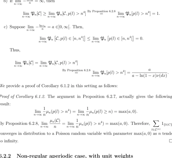
Specifically, we consider the conditional probability of the event C with respect to the length of the loop. It is trivially zero for loops whose length is less than the size of the graph. As the size of the graph Gn grows to infinity, it tends to 1 for length greater than m4n, where mn is the size of the graph, see Proposition 6.2.8.
In section 3 we show a stability result for the limit distribution ν of the eigenvalues of Qn according to Cauchy's interlacing theorem, see Proposition 6.3.2 and the subsequent note. In the second example we show that the empirical distributions of the eigenvalues of the transition.
The limit of the percentage of non-trivial loops containing all the vertices
The d-regular aperiodic case
By comparing a modified geometric variable with the coverage time of the coupon collector problem, we obtain a result different from Theorem 6.1.1 and an equivalent of Pn(C) if the killing rate is of order n−1, see Theorem 6.6.3 . Moreover, if Q is aperiodic, for every x∈ V there exists at least one path from x tox with an odd number of edges. Let Q be the transition matrix associated with a regularly connected graph with n vertices, degree d and weight 1. a).
The sum of γxx0, γx0x, and σ is a loop containing xw with an odd number of edges not greater than 3n. IfQn is the transition matrix associated with a regular connected aperiodic graph with vertices of degree d and n, then. We can now prove the following estimates for the lengths of the loops in Gn.
Assume that for each n ∈N+ Gn is a d-regular connected aperiodic graph with n vertices and assume that (H3) holds. a.1) If glue inf. According to theorem 1 of chapter 6 of the book [AF], the expectation of the "cover-and-return" time is bounded from above by dn(n−1).
Non-regular aperiodic case, with unit weights
TAc is the hit time for Ac and Ti+ is the first return time for i. For the definition of effective resistance and the relationship between an electrical network and a reversible Markov chain, see [LP]. Let π be the invariant probability of the Markov chain and let d(j) be the degree.
General case
In this case, one can divide the vertices into two parts as follows: fix a vertex x, set An ={y ∈ Vn : P. If one puts together the eigenvalues of Q2n|An and Q2n|Bn, you get exactly the squares of the eigenvalues of Qn. 2 for |λ| ≤1, one can still obtain a similar spectrum gap proposal to Corollary 6.2.3 by considering the aperiodic Markov chains on An and Bn.
Moreover, one can check whether the corresponding graphs satisfy (H1) and (H2).) Then we have instead of Corollary 6.2.4. For Proposition 6.2.8, one considers only even-length loops and the proof remains the same.
A stability result
The distributions of the eigenvalues of the transition matrices Qn form a narrow sequence of probability measurements on [−1,1]. To show its convergence, it is enough to show that the limits are the same for all convergent subsequences. Finally, for two probabilities ν and ν˜ on [-1,1], by comparing the derivatives of the two parts with respect to ρ, it can be shown that.
The intersection theorem can be found as Theorem 4.3.15 in [HJ90].4 We are ready to state the following consistency result. In the following we will give the proof for the first limit since the second can be proved in the same way.
Example: discrete torus
Example: the balls in a regular tree
For d ≥ 3, the distribution of eigenvalues Qd,n converges to a purely atomic distribution ν, which is supported on [−2. To prove convergence, it is enough to show that the moments of the probability distribution (νd,n)n converge as n → ∞, i.e. 5 Recall that the graph distanced(y, r) is the length of the shortest path connecting to rootr.
In the discrete circle the empirical distribution of the eigenvalues converges to the circular lawν on[−1,1]defined byν(dx) = 1{x. 6.3.2, the distribution of the eigenvalues of Q2,n converges to the circle law, since the difference between these two graphs is small.
The case of the complete graph
Let C(n) be the covering time of a simple random walk on the entire graph Kn. The sequence (C(n)−nlnn n)n converges legally to the Gumble distribution, see Section 2 of Chapter 6 in [AF]. As mentioned in [AF], the full graph example is a small version of this problem: Let T˜i(n) be the first time we have collected i coupons.
Consider a sequence of random variable ηn with the following distribution P(ηn=p) =. Similar to a), we can lim. We derive from Theorem 6.6.3 the following result about the asymptotic distribution of the number of loops covering Gn. Walsh, Markov processes, Brownian motion and time symmetry, second edition, Grundlehren der Mathematischen Wissenschaften [Fundamental Principles of Mathematical Sciences], vol.
Shiryaev, Limit theorems for stochastic processes, second ed., Grundlehren der Mathematischen Wissenschaften [Fundamental Principles of Mathematical Sciences], vol. Kes69] Harry Kesten, Hit probabilities of single points for processes with stationary independent increments, Memoirs of the American Mathematical Society, No.