[PENDING] Contribution to Flight Control Law Design and Aircraft Trajectory Tracking

(1)

HAL Id: tel-00974871

https://tel.archives-ouvertes.fr/tel-00974871

Submitted on 7 Apr 2014

HAL is a multi-disciplinary open access archive for the deposit and dissemination of sci- entific research documents, whether they are pub- lished or not. The documents may come from teaching and research institutions in France or

L’archive ouverte pluridisciplinaire HAL, est destinée au dépôt et à la diffusion de documents scientifiques de niveau recherche, publiés ou non, émanant des établissements d’enseignement et de recherche français ou étrangers, des laboratoires

Trajectory Tracking

Hakim Bouadi

To cite this version:

Hakim Bouadi. Contribution to Flight Control Law Design and Aircraft Trajectory Tracking. Auto- matic. INSA de Toulouse, 2013. English. �NNT : �. �tel-00974871�

(2)

��

� ��

��

Institut National des Sciences Appliquées de Toulouse (INSA Toulouse)

Systèmes (EDSYS)

Contribution to Flight Control Law Design and Aircraft Trajectory Tracking

Mardi 22 janvier 2013

Hakim BOUADI

Automatique

Houcine CHAFOUK Andrei DONCESCU

Xavier PRATS

Farès BOUDJ EMA Félix MORA-CAMINO

MAIAA / ENAC

(3)

Acknowledgements

This doctoral research was prepared within MAIAA laboratory of Air Transport de- partment at ENAC.

I would like to express my deepest gratitude to my thesis supervisor Professor Félix Mora-Camino for his continuous guidance and support throughout the research. His encouragement and advice led me to the right path and are greatly appreciated.

I would like also to thank all the members of my jury, especially Professor Farès Boud- jema from the National Polytechnic School of Algiers and Professor Francisco Javier Saez Nieto from the Polytechnic University of Madrid for their acceptance to review my thesis dissertation. Also, I would like to thank Professor Houcine Chafouk from the University of Rouen for his acceptance to chair the jury of the defense of my thesis.

My heartfelt appreciation also goes to the friends and colleagues at the Automation Research Group. They made my life at MAIAA an enjoyable and memorable experience.

I would like to thank particularly Doctor Antoine Drouin for his encouragement, advice and corrections which he and his wife Agathe have brought back to my thesis dissertation.

I would also like to extend my deepest gratitude to my family for their unconditional love and support.

I am also grateful to everyone who, in one way or another, has helped me get through these years.

(4)

3

To my parents...

To my wife...

To my daughter Maria Inès and my son Mohamed Ishaq

(5)

Résumé

Compte tenu de la forte croissance du trafic aérien aussi bien dans les pays émergents que dans les pays développés soutenue durant ces dernières décennies, la satisfaction des exigences relatives à la sécurité et à l’environnement nécessite le développement de nouveaux systèmes de guidage.

L’objectif principal de cette thèse est de contribuer à la synthèse d’une nouvelle génération de lois de guidage pour les avions de transport présentant de meilleures performances en terme de suivi de trajectoire. Il s’agit en particulier d’évaluer la faisabilité et les performances d’un système de guidage utilisant un référentiel spatial. Avant de présenter les principales approches utilisées pour le développement de lois de commande pour les systèmes de pilotage et de guidage automatiques et la génération de directives de guidage par le système de gestion du vol, la dynamique du vol d’un avion de transport est modélisée en prenant en compte d’une manière explicite les composantes du vent. Ensuite, l’intérêt de l’application de la commande adaptative dans le domaine de la con- duite automatique du vol est discuté et une loi de commande adaptative pour le suivi de pente est proposée. Les principales techniques de commande non linéaires reconnues d’intérêt pour le suivi de trajectoire sont alors analysées. Finalement, une loi de commande référencée dans l’espace pour le guidage vertical d’un avion de transport est développée et est comparée avec l’approche temporelle classique. L’objectif est de réduire les erreurs de poursuite et mieux répondre aux contraintes de temps de passage en certains points de l’espace ainsi qu’à une possible contrainte de temps d’arrivée.

Mots clé: commande automatique du vol, suivi de trajectoire, commande adaptative, commande non linéaire spatiale.

(6)

5

Abstract

Safety and environmental considerations in air transportation urge today for the development of new guidance systems with improved accuracy for spatial and temporal trajectory tracking.

The main objectives of this thesis dissertation is to contribute to the synthesis of a new generation of nonlinear guidance control laws for transportation aircraft presenting enhanced trajectory tracking performances and to explore the feasibility and performances of a flight guidance system developed within a space-indexed reference with the aim of reducing tracking errors and ensuring the satisfaction of overfly time constraints as well as final arrival time constraint. Before presenting the main approaches for the design of control laws for autopilots and autoguidance systems devoted to transport aircraft and the way current Flight Management Systems generates guidance directives, flight dynamics of transportation aircraft, including explicitly the wind components, are presented. Then, the interest for adaptive flight control is discussed and a self contained adaptive flight path tracking control for various flight conditions taking into account automatically the possible aerodynamic and thrust parametric changes is proposed. Then, the main recognized nonlinear control approaches suitable for trajectory tracking are analyzed. Finally an original vertical space-indexed guidance control law devoted to aircraft trajectory tracking is developed and compared with the classical time-indexed approach.

Key words: flight control, trajectory tracking, adaptive control, space-indexed nonlinear control.

(7)

(8)

Contents

1 General Introduction 1

2 Aircraft Flight Dynamics 5

2.1 Introduction . . . 5

2.2 Assumptions for flight dynamics modeling . . . 6

2.3 Reference frames . . . 7

2.3.1 Reference frame types . . . 7

2.3.2 Rotation matrices between frames . . . 9

2.4 The equations of motion . . . 11

2.4.1 Equations of motion in the Earth-fixed reference frame R_E 12 2.4.2 Equations of motion in the wind reference frame R_W . . . 22

2.5 Partial flight dynamics equations . . . 26

2.5.1 Longitudinal equations of motion . . . 27

2.5.2 Lateral equations of motion . . . 29

2.6 Conclusion . . . 30

3 Classical Flight Control Law Design 31 3.1 Introduction . . . 31

3.2 Classical approach to flight control law synthesis . . . 31 3.2.1 Basic principles adopted for flight control law synthesis . 32 3.2.2 Examples of implementation of the basic design principles 35

(9)

3.3 Recent approaches for longitudinal control law synthesis . . . 36

3.3.1 Modal control . . . 36

3.3.2 A reference model for longitudinal flight dynamics . . . . 39

3.3.3 Classical linear approach for flight control law synthesis . 40 3.4 Flight management generation of guidance directives . . . 43

3.4.1 FMS lateral guidance . . . 43

3.4.2 FMS vertical guidance . . . 46

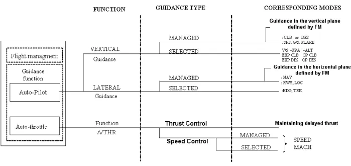
3.5 Current realizations of flight control modes . . . 48

4 Elements in Adaptive Control 53 4.1 Introduction . . . 53

4.2 The need for adaptive control . . . 55

4.3 Main adaptive control structures . . . 58

4.4 Main adaptive control techniques . . . 61

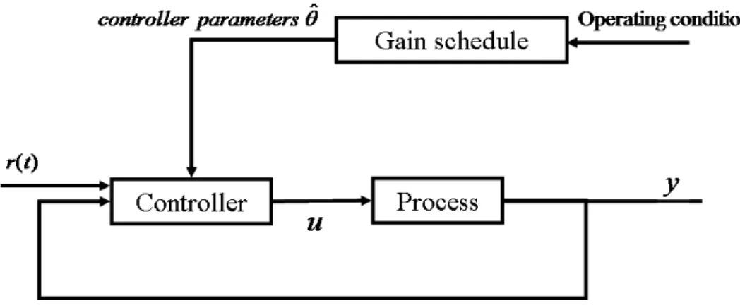
4.4.1 Gain scheduling . . . 61

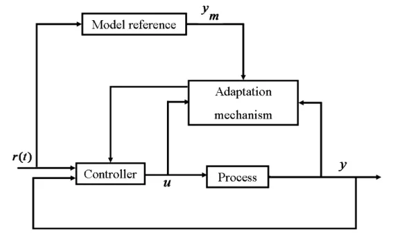
4.4.2 Model reference adaptive control (MRAC) . . . 62

4.4.3 Self-tuning regulator (STR) . . . 64

4.4.4 Dual adaptive control . . . 67

4.4.5 Adaptive control based on neural networks . . . 69

4.5 Illustrative examples . . . 70

4.5.1 MRAC for a first order linear system . . . 70

4.5.2 MRAC based feedback linearization for a class of a second order nonlinear systems . . . 77

5 A Nonlinear Adaptive Approach to Flight Path Angle Control 83 5.1 Introduction . . . 83

5.2 Vertical flight dynamics modeling . . . 85

(10)

List of Figures

2.1 Aircraft reference frames . . . 9

2.2 Euler angles configuration . . . 11

3.1 Frequency decoupling and causality . . . 34

3.2 Structural representation of controlled system . . . 38

3.3 Example of input output decoupling four order system . . . 39

3.4 Actual guidance types and corresponding modes . . . 49

4.1 Longitudinal aircraft configuration . . . 56

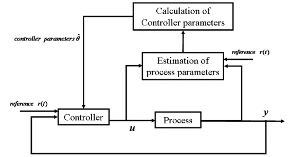
4.2 Bloc diagram of indirect adaptive control structure . . . 59

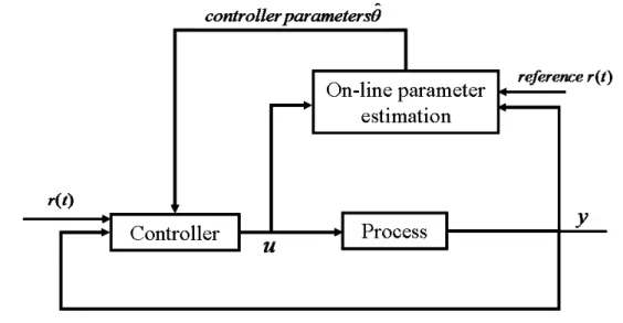
4.3 Bloc diagram of direct adaptive control structure . . . 60

4.4 Bloc diagram of system with gain scheduling . . . 62

4.5 Bloc diagram of direct model reference adaptive control (MRAC) . . . 63

4.6 Bloc diagram of indirect adaptive self-tuning control . . . 65

4.7 Bloc diagram of dual adaptive control . . . 68

4.8 Bloc diagram of neural adaptive control . . . 69

4.9 Full state-based adaptive neural control structure . . . 70

4.10 MRAC Trajectory tracking performance. . . 72

4.11 Tracking error evolution according to gain adaptation. . . 72

4.12 θ₁ parameter estimation performance. . . 73

4.13 θ₂ parameter estimation performance. . . 73

4.14 MRAC Trajectory tracking performance (MIT rule). . . 75

(15)

4.16 θ₁ parameter estimation performance (MIT rule). . . 75

4.17 θ₂ parameter estimation performance (MIT rule). . . 75

4.18 MRAC Trajectory tracking performance (MIT rule, γ = 9). . . 76

4.20 θ₁ parameter estimation performance (MIT rule, γ = 9). . . 76

4.21 θ₂ parameter estimation performance (MIT rule, γ = 9). . . 76

4.22 Trajectory tracking performance (a), tracking error (b), parameter estimation (c) and error estimation (d), respectively. . . 81

5.1 Longitudinal flight dynamics structure . . . 88

5.2 Proposed flight control structure . . . 88

5.3 Flight path angle (a) and airspeed (b) tracking performances for FC1. . . . 96

5.4 Pitch angle (a), pitch rate (b) and angle of attack (c) evolution for FC1. . 96

5.5 Control inputs: elevator deflection δ_e (a) and throttle setting δ_th (b) for FC1. 96 5.6 Controller parameters estimation related to FC1. . . 96

5.13 Control inputs: elevator deflection δe (a) and throttle setting δth (b) for FC3. 98 5.14 Controller parameters estimation related to FC3. . . 98

6.1 NDI controller structure . . . 109

(16)

LIST OF FIGURES

6.2 Altitude and airspeed tracking performances by NDI. . . 114

6.3 Angle of attack, pitch and flight path angles evolution. . . 114

6.4 Control inputs . . . 115

6.5 Aircraft piloting/Guidance system structure . . . 128

6.6 Effects diagram of guidance dynamicsθ, φ, N₁ . . . 130

7.1 Aircraft forces . . . 134

7.2 Control synoptic scheme . . . 142

7.3 Altitude trajectory tracking performance by space NDI (No wind). . . 150

7.4 Altitude trajectory tracking performance by time NDI (No wind). . . 150

7.5 Initial altitude tracking by space NDI (No wind). . . 150

7.6 Initial altitude tracking by time NDI (No wind). . . 150

7.7 Airspeed profile tracking performance by space NDI (No wind). . . 151

7.8 Airspeed profile tracking performance by time NDI (No wind). . . 151

7.9 Angle of attack and flight path angle evolution with space NDI (a,b), (No wind). . . 151

7.10 Angle of attack and flight path angle evolution with time NDI (c,d), (No wind). . . 151

7.11 Control inputs with space NDI (a,b), (No wind). . . 152

7.12 Control inputs with time NDI (c,d), (No wind). . . 152

7.13 Delayed initial situation and recover . . . 152

7.14 Advanced initial situation and recover . . . 153

7.15 Example of wind components realization . . . 153

7.16 Delayed initial situation and recover with wind . . . 154

7.17 Advanced initial situation and recover with wind . . . 155

A.1 ISA temperature and pressure profiles . . . 164

(17)

(18)

List of Tables

3.1 Assignment of control channels to piloting/guidance modes . . . 33

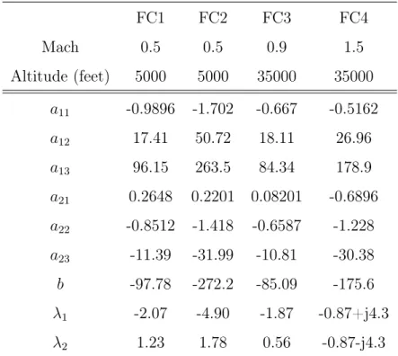
3.2 Example of values for the aerodynamic derivatives of a wide body aircraft . 41 4.1 Parameter values for different flight conditions . . . 57

5.1 Flight conditions . . . 93

5.2 Aircraft general parameters . . . 94

5.3 Weight and inertias . . . 94

A.1 ISA Constants . . . 161

A.2 Data for ISA . . . 164

(19)

(20)

Chapter 1

General Introduction

World air transportation traffic has known a sustained increase over the last decades lead- ing to airspace near saturation in large areas of developed and emerging countries. For example, today up to 27,000 flights cross European airspace every day while the number of passengers is expected to double by 2020. Then safety and environmental considerations urge today for the development of new guidance systems with improved accuracy for spatial and temporal trajectory tracking. Available infrastructure of current ATM (Air Traffic Management) system will no longer be able to stand this growing demand unless breakthrough improvements are made.

In the future Air Traffic Management environment which will be the result of huge research projects such as SESAR (Single European Sky ATM Research) and NextGen (Next Generation Air Transportation System), two main objectives are targeted, strategic data link services for sharing of information and negotiation of planning constraints between ATC (Air Traffic Control) and the aircraft in order to ensure planning consistency and the use of the 4D aircraft trajectory information in the Flight Management System for ATC operations

Current Civil Aviation guidance systems operate with real time corrective actions to maintain the aircraft trajectory as close as possible to the planned trajectory or to follow timely ATC tactical demands based either on spatial or temporal considerations [Miele

(21)

et al., 1986a, Miele et al., 1986b]. While wind remains one of the main causes of guidance errors [Miele, 1990, Psiaki and Stengel, 1985, Psiaki and Park, 1992], these news solicita- tions by ATC are attended with relative efficiency by current airborne guidance systems.

However, these guidance errors are detected for correction by navigation systems whose accuracy has known large improvements in the last decade with the hybridization of inertial units with satellite information. Nevertheless, until today vertical guidance remains problematic [Singh and Rugh, 1972a, Stengel, 1993] and corresponding covariance errors [Sandeep and Stengel, 1996] are still large, considering the time-based control laws which are applied by flight guidance systems [Psiaki and Park, 1992, Psiaki, 1987].

The main objective of this thesis dissertation is to contribute to the synthesis of a new generation of nonlinear guidance control laws for transportation aircraft presenting enhanced tracking performances.

The flight dynamics of a transportation aircraft is nonlinear and subject to many changes especially while performing climb or descent manoeuvers and subject to external perturbations such as wind turbulence. Today, the unique certified adaptive control technique implemented on board aircraft autopilots to cope with these changes is gain scheduling. In fact, this technique uses an off-line parameters estimation approach which can show some weaknesses in certain flight conditions and situations. However, one of the main objectives of the present research work is to propose a self contained adaptive control technique [Bouadi et al., 2011] which will be able to take into account automatically the possible aerodynamic and thrust parametric changes using an on-line approach integrating parameters estimation.

While the construction of flight plans for transportation aircraft by the Flight Manage- ment System (FMS) are space-indexed to take into account space restrictions and to locate specific flight plan events (Top of Climb (T/C), Top of Descent (T/D)) and some overfly time constraints and final arrival time constraints must be also satisfied when taking into consideration the real operational air traffic environment. Today this kind of constraints are in general managed by tuning some tactical parameters such as the Cost Index (CI) within the Flight Management System (FMS) or by modifying the flight profile, both in a

(22)

rather heuristic way.

When considering current guidance systems for transportation aircraft, they are in general tuned in a time index context while in many situations the trajectory to be followed is defined with respect to space. This is the case for Continuous Descent Approaches (CDA’s) as well as for take-off and approach trajectories designed with a noise abattment purpose. This has of course consequences on the Flight Technical Error (FTE) developed by these aircraft.

The second main objective of this thesis is to explore the feasibility and eventually the performances of a flight guidance system developed within a space-indexed reference [Bouadi et al., 2012, Bouadi and Mora-Camino, 2012a] which should present reduced tracking errors and be able to meet more easily overfly time constraints as well as a final arrival time constraint.

In order to better present our efforts and findings towards the two main objectives of this research, the manuscript is organized as follows:

The first chapter of this thesis dissertation is devoted to introduce mathematical models describing the flight dynamics of a transportation aircraft with a set of nonlinear differential equations. These classical equations have been respectively displayed in the body reference frame and in the wind reference frame where the wind components are here explicitly taken into account.

In the second chapter we introduce the main approaches which have been developed in the past decades for the design of control laws for autopilots and autoguidance systems devoted to transport aircraft. Then, the way the Flight Management System (FMS) generates guidance directives is discussed while current flight control modes encountered in a modern transportation aircraft are described and finally some of the main limitations of current flight control law design approaches are pointed out.

The third chapter of this thesis dissertation is devoted to show the interest of adaptive control for flight control applications. Then, the main adaptive control structures and techniques available today are reviewed. After, one of the more popular adaptive control approach, the Model Reference Adaptive Control (MRAC), is applied for two illustrative

(23)

examples.

In the fourth chapter the (MRAC) approach is extended to develop a nonlinear adaptive control scheme to ensure accurate flight path angle control for a transportation aircraft while maintaining its desired airspeed and this for various flight conditions. Considered cases such as go-around and obstacle avoidance situations illustrate the ability of the proposed solution to cope with extreme flight conditions.

In the fifth chapter, the three main recognized nonlinear control approaches suitable for trajectory tracking (Nonlinear Dynamic Inversion, Backstepping and Differential Flatness) are introduced and their respective applicability for aircraft trajectory tracking is discussed.

In the sixth chapter, the problem of designing vertical guidance control laws with the aim of improving aircraft vertical tracking accuracy and ensuring the satisfaction of overfly time constraints is treated. With this objective a new space-indexed representation of aircraft vertical guidance dynamics is introduced and a spatial nonlinear dynamic inversion control law is proposed to make the aircraft follow accurately desired vertical profiles and airspeeds. The results of this new approach are compared to those obtained from a classical (temporal) nonlinear dynamic inversion control law.

The general conclusion of this thesis summarize the main efforts developed in this research work before displaying its main contributions to flight control law design techniques.

Finally some perspectives to pursue this research line are discussed.

(24)

Chapter 2

Aircraft Flight Dynamics

2.1 Introduction

The objective of this chapter is to introduce mathematical models describing the flight dynamics of a general aircraft to give ground to our study considering flight control objectives.

The dynamic behavior of a transportation aircraft, considered as a rigid body with six degrees of freedom within a quasi-stationary aerodynamic flow field, can be described by a set of analytical nonlinear differential equations where aerodynamic effects are reduced to global forces and moments.

This set of nonlinear differential equations is called the complete mathematical aircraft model although many subsystems (engines, control channels dynamics) are bypassed. In many articles dealing with flight dynamics [Etkin and Reid, 1996, Etkin, 1985, Nelson, 1998, McLean, 1990], this kind of model represents the basis for the analysis of aircraft dynamic behavior. Simplified versions of this model have been used to propose solution to different flight control problems. It is for example the case when control laws are synthesized from linearized versions of the flight dynamics model. The validity of these simple and approximative mathematical models is restricted to a limited domain around the reference point of the flight domain used in the linearization process. As a consequence,

(25)

a large number of approximate models can be required in order to cover all design aspects, rendering the approach rather cumbersome.

New results in control theory [Stengel, 2004]have turned feasible quite recently the use of nonlinear aircraft mathematical models in the design of effective flight control systems.

Before starting the development of the whole set of nonlinear differential equations describing flight dynamics of a transportation aircraft taking especially into account wind components, we present the assumptions adopted to develop a tracktable and representa- tive model of the dynamics of a transportation aircraft. Then, the main reference frames used in flight dynamics modeling are introduced as well as the different transformation matrices allowing the transition between reference-frames. The differential nonlinear equations derived from the second dynamics laws (Newton’s principle) are developed considering explicitly the presence of wind.

Finally, the equations of the nonlinear longitudinal motion dynamics on one side and those describing the nonlinear lateral dynamics on the other side are described in detail since traditionally many flight control problems have been split into longitudinal and lateral ones considering little coupling between them.

2.2 Assumptions for flight dynamics modeling

For better understanding of the aircraft flight dynamics developed in the next section, the working assumptions are as follows:

1. The Earth is supposed:

• The Earth coordinate system is assumed to be inertial,

• Flat, and

• The vector of gravity is constant.

2. The atmosphere is supposed standard:

• Dry,

(26)

2.3. REFERENCE FRAMES

• Stable, and

• It is a function of the altitude.

3. Compressibility:

• No chock wave below the critical Mach number,

• High increase of drag force above the critical Mach.

4. Main aircraft characteristics:

• The aircraft mass,

• The aircraft is supposed symmetric,

• Aircraft is assumed a rigid body with center of gravity COG.

2.3 Reference frames

2.3.1 Reference frame types

To describe both the position and the behavior of an aircraft, we need a reference frame (RF). There are several reference frames. Which one is most convenient to use depends on the circumstances. We will examine a few.

• First let us examine theinertial reference frameR_I, it is a right-handed orthogonal system. Its origin A is the center of the Earth. The Z_I axis points North. The X_I axis points towards the vernal equinox. The Y_I axis is perpendicular to both of them. Its direction can be determined using the right-hand rule. For flight dynamics applications the Earth axes are generally of minimal use, and hence will be ignored.

The motions relevant to dynamic stability are usually too short in duration for the motion of the Earth itself to be considered relevant for aircraft.

• In the (local) Earth-fixed reference frame R_E, the origine O is at an arbitrary location on the ground. the Z_E axis points towards the ground. The X_E axis is

(27)

directed North and it is perpendicular to the Z_E axis. The Y_E axis can again be determined using the right-hand rule.

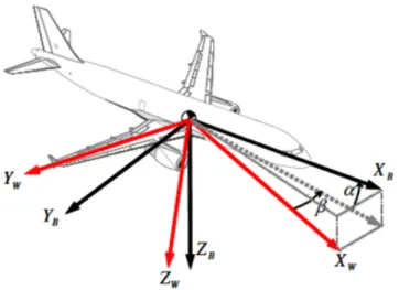
• Thebody reference frameR_Bis often used when dealing with aircraft. The origin of the reference frame is the center of gravity (COG) of the aircraft. TheX_B axis lies in the symmetry plane of the aircraft and points forward. The Z_B axis also lies in the symmetry plane, but points downward. The Y_B axis is perpendicular to theX_B axis and can again be determined using the right-hand rule. Sometimes we choose the body axes to be aligned with the vehicle principle axes. The origin is generally taken at the aircraft center of gravity or at a fixed reference location relative to the geometry.

• Thestability reference frameR_S is similar to the body-fixed reference frameR_B. It is rotated by an angle of attackα about theY_B axis. To find this angleα, we must examine the relative wind vector. We can project this vector onto the plane of symmetry of the aircraft. This projection is then the direction of the X_S axis. The Z_S axis still lies in the plane of symmetry. Also, the Y_S axis is still equal to the Y_B axis. So, the relative wind vector lies in the X_SY_S plane. This reference frame is particularly useful when analyzing flight dynamics.

• Theaerodynamic or wind reference frameR_W is similar to the stability reference frameR_S. It is rotated by sideslip angleβ about theZ_S axis. This is done, such that the X_W axis points in the direction of the relative wind vector V_a. So the X_W axis generally does not lie in the sysmmetry plane anymore. TheZ_W axis is still equation to the Z_S axis. TheY_W axis can now be found using the right-hand rule.

• Finally, there is the vehicle reference frame R_V. Contrary to the other systems, this is a left-handed system. Its origin is a fixed point on the aircraft. The X_V axis points to the rear of the aircraft. TheY_V axis points to the left. Finally, theZ_V axis can be found using the left-hand rule. (It points upward.) This system is often used by the aircraft manufacturer, to denote the position of parts within the aircraft.

(28)

2.3. REFERENCE FRAMES

Figure 2.1: Aircraft reference frames

2.3.2 Rotation matrices between frames

Based on what has been described above, we can go from one reference frame to any other reference frame, using at most three Euler angles. An Euler angle can be represented by a transformation matrix T. To see how it works, let us consider a vector x¹ in reference frame 1. The matrix T21 now calculates the coordinates of the same vectorx² in reference frame 2, according to:

x² =T21x¹ (2.3.1)

Let us suppose we are only rotating about the X axis. In this case, the transformation matrix T²¹ is quite simple. In fact, it is:

T²¹ =







1 0 0

0 cosφx sinφx

0 −sinφ_x cosφ_x







(2.3.2)

Similarly, we can rotate about the Y axis and theZ axis. In this case, the transformation matrices are, respectively:

T21=







cosφ_y 0 −sinφ_y

0 1 0

sinφ_y 0 cosφ_y







and T21=







cosφ_z sinφ_z 0

−sinφ_z cosφ_z 0

0 0 1







(2.3.3)

(29)

Rotation matrices have interesting properties. They only rotate points. They do not deform them. For this reason, the matrix columns are orthogonal and, because the space is not stretched out either, these columns must also have length 1. A transformation matrix is thus orthogonal. This implies that:

T⁻¹21 =T^T21 =T12 (2.3.4)

However, to define the transformation matrix which allows the transition between the three body centered reference frames: the body reference frame R_B, the stability reference frame R_S and the wind reference frame R_W represented on the fig.(2.1), we proceed first at the body reference frame R_B. If we rotate this frame by an angle of attack α around the Y_B axis, we find the stability reference frame R_S. If we then rotate it by the sideslip angle β around theZ_B axis, we get the wind reference frame R_W. So we can find that:

X_W =







cosβ sinβ 0

−sinβ cosβ 0

0 0 1





 X_S =







cosβ sinβ 0

−sinβ cosβ 0

0 0 1













cosα 0 −sinα

0 1 0

−sinα 0 cosα





 X_B

(2.3.5) by working things out, it appears that the transformation matrix allowing the transition between the body-fixed reference frame RB and wind reference frame RW is as follows:

T^{W B} =







cosβcosα sinβ cosβsinα

−sinβcosα cosβ −sinβsinα

−sinα 0 cosα







(2.3.6)

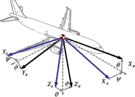
We can perform a similar transformation between the Earth-fixed reference frame R_E and the body-fixed reference frame R_B. To do that, we first have to rotate over the yaw angle ψ about the Z_B axis. We then rotate over the pitch angle θ about the resulting Y axis. Finally, the new resulting reference frame is then rotated over the roll angleφ around itsX axis. It results the configuration shown infig.(2.2). Then, the transformation matrix

(30)

2.4. THE EQUATIONS OF MOTION

Figure 2.2: Euler angles configuration TBE is such as:

TBE =







cosθcosψ cosθsinψ −sinθ

sinφsinθcosψ−cosφsinψ sinφsinθsinψ+ cosφcosψ sinφcosθ cosφsinθcosψ+ sinφsinψ cosφsinθsinψ−sinφcosψ cosφcosθ







(2.3.7)

When analyzing the flight dynamics, we are concerned both with rotation and trans- lation of this axis set with respect to a fixed inertial reference frame. For all practice purposes, the local Earth-fixed reference frame R_E is used.

2.4 The equations of motion

In this section the aircraft dynamics is studied. We present the governing equations linking the variables to be controlled to the control inputs available to us. With respect to several references in literature [Stevens and Lewis, 2003], the presentation is focused on arriving at a mathematical model suitable for control design, consisting of a set of first order nonlinear differential equations. For a deeper insight into the mechanics and aerodynamics

(31)

behind the model, the reader is referred to the aformentioned references [Etkin and Reid, 1996, McLean, 1990, Nelson, 1998].

2.4.1 Equations of motion in the Earth-fixed reference frame R

_E

The flight dynamics of an aircraft are described by its equations of motion. First, we will use the assumptions that Earth is flat and fixed, and that the aircraft body is rigid. This yields a six (06) degrees of freedom model. The dynamics can be described by a state space model with twelve (12) states.

Before let us define:

• P_Ac = (P_N, P_E, h)^T, the aircraft position expressed in the Earth-fixed reference frame R_E.

• V_I = (u, v, w)^T, the inertial speed vector expressed in the body reference frame R_B.

• Va = (u−wX, v−wY, w−wZ)^T, the airspeed vector expressed in the body reference frame.

• Φ = (φ, θ, ψ)^T, the Euler angles describing the orientation of the aircraft relative to the Earth-fixed reference frame.

• Ω = (p, q, r)^T, the angular velocity of the aircraft expressed in the body-fixed reference frame.

where (w_X, w_Y, w_Z) are the components of the wind vector expressed in the body-fixed frame such as:





 w_X w_Y w_Z







=T^BE





 W_x W_y W_z







(2.4.1)

The only coupling from P_Ac to other state variables is through the altitude dependance of the aerodynamic pressure. The equations governing the remaining three state vectors

(32)

2.4. THE EQUATIONS OF MOTION

can be compactly written as:

F =mdV_I

dt |_B+mΩ|_BE ×V_I (2.4.2a)

M_G=IG

dΩ_BE

dt |_B+ Ω_BE ×IGΩ_BE (2.4.2b)

Φ =˙ E(Φ)Ω|_BE (2.4.2c)

where

E(Φ) =







1 sinφtanθ cosφtanθ 0 cosφ −sinφ 0 tanθ ^cos_cos^φ_θ







(2.4.3)

m is the aircraft mass and IG is the aircraft inertia matrix. The forces and moments equations follow from applying the formalism of Newton and the attitude equation results from the relation between the Earth-fixed and the body-fixed reference frames.

F and M_G represent respectively the sum of the forces and moments acting on the aircraft at the center of gravity. These forces and moments appear from three major sources:

• gravity,

• engine thrust, and

• aerodynamic efforts.

Introducing:

F =FG+FE +FA (2.4.4a)

MG =ME+MA (2.4.4b)

Forces

To establish the aircraft equations of motion, we start by examining forces. Our starting point is Newton⁰s second law. However, Newton⁰s second law only holds in an inertial reference frame. Luckily, the assumptions we have made earlier imply that the Earth-fixed

(33)

reference frame R_E is inertial. However, R_B is not an inertial reference frame. So we will derive the equations of motion with respect to RE.

Let⁰s examine an aircraft. Newton⁰s second law states that:

F = Z

dF = d dt

Z

V_pdm

(2.4.5) By integrating over the entire body, it can be shown that the right side of this equation equals _dt^d(mV_I), where V_I is the velocity of the center of gravity of the aircraft. If the aircraft has a constant mass, we can rewrite the above equation into:

F =mdVI

dt =mA_G (2.4.6)

But it does imply something very importatnt. The acceleration of the center of gravity of the aircraft does not depend on how the forces are distributed along the aircraft. It only depends on the magnitude and direction of the forces.

There is one slight problem. The above equation (2.4.6) is expressed in the Earth reference frame. But we usually work in the body-fixed reference frame R_B. So we need to convert it. To do this, we can use the rules related to the relative motion:

AG= dV_I

dt |E = dV_I

dt |B+ ΩBE ×VI (2.4.7)

inserting (2.4.7) into the above equation (2.4.6) will give:

F =mdVI

dt |_B+mΩ_BE ×V_I =m







˙

u+qw−rv

˙

v+ru−pw

˙

w+pv−qu







(2.4.8)

As it is mentioned above, the main forces acting on the aircraft body are gravity, engine thrust and aerodynamic efforts forces. Grvaity only gives a force contribution since it acts at the aircraft center of gravity. The gravitational force, mg, directed along the normal of the Earth plane, is considered constant over the altitude envelope. This yields:

F_G =







−mgsinθ mgsinφcosθ mgcosφcosθ







(2.4.9)

(34)

2.4. THE EQUATIONS OF MOTION

The thrust force due to the propulsion system can have components that act along each of the body-fixed reference frame RB. Assuming the engine to be positioned so that the thrust acts parallel to the aircraft bodyX-axis, yields:

F_E =





 F_T

0 0







(2.4.10)

The aerodynamic forces and moments, or aerodynamic efforts, result due to the in- teraction between the aircraft body and the incoming airflow. The size and direction of the aerodynamic efforts are determined by the amount of air diverted by the aircraft in different directions [Etkin and Reid, 1996]. The amount of air diverted by the aircraft is mainly decided by:

• the speed and density of the airflow(V_a, ρ),

• the geometry of the aircraft (δa, δe, δr, S, c, b),

• the orientation of the aircraft relative to the airflow (α, β)

The aerodynamic efforts also depend on other variables, like the angular rates (p, q, r) and the time derivatives of the aerodynamic angles ( ˙α,β), but these effects are not as˙ pronounced.

This motivates the standard way of modeling aerodynamic forces and moments:

Force=qSC_F(δ_a, δ_e, δ_r, δ_th, α, β, p, q, r,α,˙ β, ...)˙ Moment=qSlC_M(δ_a, δ_e, δ_r, δ_th, α, β, p, q, r,α,˙ β, ...)˙

where δ_a, δ_e, δ_r and δ_th are respectively aileron, elevator, rudder deflections and throttle setting and q denotes the aerodynamic pressure and it is expressed such as:

q= 1

2ρ(h)V_a² (2.4.12)

and captures the density dependance and most of the speed dependance, S is the aircraft wing surface area andl refers to the length of the lever arm connected to the moment. C_F

(35)

and C_M are known as aerodynamic coefficients. These are difficult to model analytically but can be estimated empirically through wind tunnel experiments and actual flight tests.

Typically, each coefficient is written as a sum of several components, each capturing the dependance of one or more of the variables above. These components can be represented in several ways. A common approach is to store them in look-up tables and use interpolation to compute intermediate values. In other approaches one tries to fit the data to some parameterized function.

In the body-fixed reference frame RB, we have the expressions:

F_A=





 F_X F_Y F_Z







(2.4.13)

where

F_X = 1

2ρ(h)V_a²SC_x (2.4.14a) F_Y = 1

2ρ(h)V_a²SC_y (2.4.14b) F_Z = 1

2ρ(h)V_a²SC_z (2.4.14c) By combining equations (2.4.9), (2.4.10) and (2.4.13) with the equation of motion for forces (2.4.8), we find that:

˙

u=rv−qw−gsinθ+ F_X +F_T

m (2.4.15a)

˙

v =pw−ru+gsinφcosθ+ FY

m (2.4.15b)

˙

w=qu−pv+gcosφcosθ+F_Z

m (2.4.15c)

Moments

Before starting to study the moments acting on the aircraft, we first examine angular momentum. The angular momentum of an aircraftB_Gwith respect to the center of gravity is defined as:

B_G= Z

dB_G =r×V_pdm (2.4.16)

(36)

2.4. THE EQUATIONS OF MOTION

where we integrate over every point P in the aircraft. We can substitute:

V_p =V_I+dr

dt|_B+ Ω_BE ×r (2.4.17)

if we insert (2.4.17) in equation (2.4.16), we can eventually find that:

B_G =IGΩ_BE (2.4.18)

As it is indicated before the matrixI^G is the aircraft inertia matrix, with respect to the center of gravity. It is defined as follows:

I^G =







I_xx −I_xy −I_xz

−Ixy Iyy −Iyz

−I_xz −I_yz I_zz







=







R (r_y²+r²_z)dm −R

(r_xr_y)dm −R

(r_xr_z)dm

−R

(rxry)dm R

(r_x²+r²_z)dm −R

(ryrz)dm

−R

(r_xr_z)dm −R

(r_yr_z)dm R

(r_x²+r²_y)dm





 (2.4.19) we have assumed that theXZ-plane of the aircraft is a plane of symmetry. For this reason, I_xy =I_yz = 0.

The moment acting on the aircraft expressed in the Earth-fixed reference frame supposed inertial, with respect to its center of gravity, is given by:

M_G = Z

dM_G = Z

r×dF = Z

r× d(V_pdm)

dt (2.4.20)

where we integrate over the entire body, we can simplify the above relation to:

MG = dBG

dt |E (2.4.21)

The above relation only holds for inertial reference frames. However, we want to have the above relation in R_B. So we rewrite it to:

M_G= dB_G

dt |_B+ Ω_BE ×B_G (2.4.22)

and by using (2.4.18), we can continue to rewrite the above equation. We find the equation (2.4.4b) which in matrix-form can be written as:

M_G =







I_xxp˙+ (I_zz−I_yy)qr−I_xz(pq+ ˙r) I_yyq˙+ (I_xx−I_zz)pr+I_xz(p²−r²)

I_zzr˙+ (I_yy−I_xx)pq+I_xz(qr−p)˙







(2.4.23)

(37)

Note that we have used the fact that I_xy =I_yz = 0.

To define the external moments, we can distinguish two types of moments, acting on the aircraft. There are moments caused by gravity, and moments caused by aerodynamic forces. The moments caused by gravity are zero since the resultant gravitational force acts in the aircraft center of gravity. So we only need to consider the moments caused by aerodynamic forces. We denote those as:

M_A=





 L M N







(2.4.24)

where L, M and N denote respectively, the rolling moment, the pitching moment and yawing moment and they are expressed in the body-fixed reference frame such as:

L= 1

2ρ(h)V_a²SbC_l (2.4.25a) M = 1

2ρ(h)V_a²ScC_m (2.4.25b) N = 1

2ρ(h)V_a²SbC_n (2.4.25c) with C_l, C_m and C_n represent the aerodynamic moments coefficients. They are expressed such as:

C_l =C_l₀ +C_l_ββ+C_l_r rb

2V_a +C_l_p pb

2V_a +C_l_δaδ_a+C_l_δrδ_r (2.4.26a) C_m =C_m₀ +C_m_αα+C_m_α_˙ αc˙

2V_a +C_m_q qc

2V_a +C_m_δeδ_e+C_m_δthδ_th (2.4.26b) C_n =C_n₀+C_n_ββ+C_n_r rb

2V_a +C_n_p pb

2V_a +C_n_δaδ_a+C_n_δrδ_r (2.4.26c) In addition, the propulsive forces can also create moments if the thrust does not act through the aircraft center of gravity. We assume the engine to be mounted so that the thrust point lies in the body-axes XZ-plane, offset from the center of gravity by ZT P in the body-axes Z-direction results in:

M_E =





 0 F_TZ_{T P}

0







(2.4.27)

(38)

2.4. THE EQUATIONS OF MOTION

By combining equations (2.4.22), (2.4.24) with the equation of motion for moments (2.4.21), we find that:

˙

p= (a₁p+a₂r)q+a₃L+a₄N (2.4.28a)

˙

q =a₅pr−a₆(p²−r²) +a₇(M +F_TZ_{T P}) (2.4.28b)

˙

r = (a₈p−a₁r)q+a₄L+a₉N (2.4.28c) Here we have introduced:

a₁ = (I_xx−I_yy+I_zz)I_xz

I_xxI_zz −I_xz² a₂ = (I_yy−I_zz)I_zz −I_xz²

I_xxI_zz −I_xz² a₃ = I_zz I_xxI_zz −I_xz²

a₄ = I_xz

IxxIzz−I_xz² a₅ = I_zz −I_xx Iyy

a₆ = I_xz Iyy

a₇ = 1 Iyy

a₈ = I_xx(I_xx−I_yy) +I_xz²

IxxIzz−I_xz² a₉ = I_xx IxxIzz−I_xz²

Translational kinematics

Since we have the force and moment equations (2.4.13) and (2.4.24), we only need to find the kinematics relations for the aircraft. First, we examine translational kinematics. This concerns the velocity of the center of gravity of the aircraft with respect to the ground.

The velocity of the center of gravity, with respect to the ground, is called the kinematic velocity Vk. It is described in the Earth-fixed reference frame RE by:

V_k=





 V_N V_E

−V_Z







(2.4.29)

where V_N is the velocity component in the Northward direction, V_E is the velocity component in the Eastward direction, and −V_Z is the vertical velocity component. Note that the minus sign is present because, in the Earth-fixed reference frame, V_Z is defined to be positive downward. However, in the body-fixed reference frame R_B, the inertial speed

(39)

vector of the center of gravity, with respect to the ground, is given by:

V_I =





 u v w







(2.4.30)

To relate those two vectors to each other, we need the transformation matrix T^BE defined in (2.3.7). This gives us:

V_k=TEBV_I =T^TBEV_I (2.4.31) This is the translational kinematic relation. We can use it to derive the change of the aircraft position. To do that, we simply have to integrate the velocities. Thus, we have:

x(t) = Z t

0

VNdt, y(t) = Z t

0

VEdt and z(t) =− Z t

0

VZdt (2.4.32) where:







˙ x

˙ y

˙ z







=







cosθcosψ sinφsinθcosψ−cosφsinψ cosφsinθcosψ+ sinφsinψ sinψcosθ sinφsinθsinψ+ cosφcosψ cosφsinθsinψ−sinφcosψ

−sinθ sinφcosθ cosφcosθ











 u v w





 (2.4.33)

Rotational kinematics

This concerns the motion of rotation of the aircraft. In the Earth-fixed reference frameR_E, the rotational velocity is described by the variablesφ,˙ θ˙andψ. However, in the body-fixed˙ frame, the rotational velocity is described by roll, pitch and yaw rates(p, q, r), respectively.

The relation between these two set of variables can be shown from the equation (2.4.2c) as follows:

φ˙ =p+ tanθ(qsinφ+rcosφ) (2.4.34a)

θ˙=qcosφ−rsinφ (2.4.34b)

ψ˙ = 1

cosθ(qsinφ+rcosφ) (2.4.34c)

(40)

2.4. THE EQUATIONS OF MOTION and inversely:





 p q r







=







1 0 −sinθ

0 cosφ sinφcosθ 0 −sinφ cosφcosθ











 φ˙ θ˙ ψ˙







(2.4.35)

Summary

The state equations which describe the aircraft translational and rotational motions expressed in the Earth-fixed reference frame are gathered such as:

1. State equations describing aircraft angular velocities:

˙

p= (a₁p+a₂r)q+a₃L+a₄N (2.4.36a)

˙

q =a₅pr−a₆(p²−r²) +a₇(M +F_TZ_{T P}) (2.4.36b)

˙

r = (a₈p−a₁r)q+a₄L+a₉N (2.4.36c) 2. State equations describing aircraft Euler angles:

φ˙ =p+ tanθ(qsinφ+rcosφ) (2.4.37a)

θ˙=qcosφ−rsinφ (2.4.37b)

ψ˙ = 1

cosθ(qsinφ+rcosφ) (2.4.37c) 3. State equations describing airspeed components:

˙

u=rv−qw−gsinθ+ F_X +F_T

m (2.4.38a)

˙

v =pw−ru+gsinφcosθ+ F_Y

m (2.4.38b)

˙

w=qu−pv+gcosφcosθ+FZ

m (2.4.38c)

4. State equations describing aircraft position:







˙ x

˙ y

˙ z







=







cosθcosψ sinφsinθcosψ−cosφsinψ cosφsinθcosψ+ sinφsinψ sinψcosθ sinφsinθsinψ+ cosφcosψ cosφsinθsinψ−sinφcosψ

−sinθ sinφcosθ cosφcosθ











 u v w





 (2.4.39)

(41)

2.4.2 Equations of motion in the wind reference frame R

W

The aerodynamic forces are also commonly expressed in the wind reference frame RW

related to the body reference frameR_B as indicated in fig.(2.1), where we have:

F_A|_W =







−D Y

−L







(2.4.40)

with L, Y and D denote respectively lift, side and drag forces. They are expressed as follows:

L= 1

2ρ(h)V_a²SC_L (2.4.41a) Y = 1

2ρ(h)V_a²SC_Y (2.4.41b) D= 1

2ρ(h)V_a²SCD (2.4.41c) where the lift, side and drag aerodynamic forces coefficients,C_L,C_Y andC_D mainly depend on the angle of attack α and sideslip angle β, respectively. Their analytical expressions depend on control objectives and they are generally presented [Etkin and Reid, 1996,Etkin, 1985, McLean, 1990] such as:

C_L=C_L₀ +C_L_αα+C_L_q q Va

+C_L_δeδ_e (2.4.42a)

C_Y =C_Y₀ +C_Y_ββ+C_Y_r rb

2V_a +C_Y_p pb

2V_a +C_Y_δrδ_r (2.4.42b) CD =CD0 +CDαα+CD_α2α² (2.4.42c) Note that, the aerodynamic forcesF_X,F_Y andF_Zcan be expressed in the wind reference frame R_W such as:

F_X =−Dcosαcosβ−Y sinβcosα+Lsinα (2.4.43a)

F_Y =−Dsinβ+Y cosβ (2.4.43b)

F_Z =−Dsinαcosβ−Y sinαsinβ−Lcosα (2.4.43c)

(42)

2.4. THE EQUATIONS OF MOTION

We can rewrite the force equations in terms of angle of attack α, sideslip angle β and airspeed Va variables by performing the following change of variables:

u=V_acosαcosβ+w_X (2.4.44a)

v =V_asinβ+w_Y (2.4.44b)

w=V_asinαcosβ+w_Z (2.4.44c)

as a first result, we can get:

V_a=p

(u−w_X)²+ (v−w_Y)²+ (w−w_Z)² (2.4.45a) α= arctan

w−w_Z u−w_X

(2.4.45b) β = arcsin

v−w_Y V_a

(2.4.45c)

Then, the equations of drag, lift and side forces expressed in the wind reference frame R_W become:

D=−F_Xcosαcosβ−F_Y sinβ−F_Zsinαcosβ (2.4.46a)

L=F_Xsinα−F_Zcosα (2.4.46b)

Y =−F_Xcosαsinβ+F_Y cosβ−F_Zsinαsinβ (2.4.46c)

where the state equations describing airspeed V_a, angle of attack α and sideslip angle β

(43)

behaviors are respectively such as:

V˙_a = 1

m(−D+F_T cosαcosβ+mg₁) +p(w_Y sinαcosβ+w_Zsinβ) +qcosβ(w_Zcosα+w_Xsinα) +r(w_X sinβ+w_Y cosαcosβ)

−w˙_Xcosαcosβ−w˙_Y sinβ−w˙_Zsinαcosβ

(2.4.47a)

˙

α =q−(pcosα+rsinα) tanβ+ 1

mVacosβ(−L−F_Tsinα+mg₂)

+ 1

V_acosβ

q(w_Zsinα+w_Xcosα)−w_Y(pcosα+rsinα) + ˙w_Xsinα−w˙_Zcosα

(2.4.47b) β˙ =psinα−rcosα+ 1

mV_a(Y −F_Tcosαsinβ+mg₃) + 1 V_a

−w_X(qsinαsinβ+rcosβ) +w_Y sinβ(psinα−rcosα) +w_Z(qcosαsinβ+pcosβ) + ˙w_Xcosαsinβ

−w˙Y cosβ+ ˙wZsinαsinβ

(2.4.47c) with the contributions g₁,g₂ and g₃ due to the gravity are given by:

g₁ =g(−cosαcosβsinθ+ sinβcosθsinφ+ sinαcosβcosθcosφ) (2.4.48a) g₂ =g(cosαcosθcosφ+ sinαsinθ) (2.4.48b) g₃ =g(cosβcosθsinφ+ cosαsinβsinθ−sinαsinβcosθcosφ) (2.4.48c)

In no wind condition, airspeed, angle of attack and sideslip angle equations are:

V˙_a= 1

m(−D+F_T cosαcosβ+mg₁) (2.4.49a)

˙

α=q−(pcosα+rsinα) tanβ+ 1

mVacosβ(−L−F_T sinα+mg₂) (2.4.49b) β˙ =psinα−rcosα+ 1

mV_a(Y −F_T cosαsinβ+mg₃) (2.4.49c) For flight path angles, the mathematical expressions are derived as follows:

V~_I =V~_a+W~ (2.4.50)

(44)

2.4. THE EQUATIONS OF MOTION

whereV~_I,V~_a and W~ are respectively the inertial, the airspeed and the wind speed vectors.

The components of the inertial airspeed vector expressed in the Earth frame are such as:

V~_I =







VIcosγIcosµ V_Icosγ_Isinµ

−VIsinγI







(2.4.51)

where V_I =

−

→V_I

, γ_I is the inertial path angle and µ is the horizontal orientation of the inertial speed. The airspeed vecto

[PENDING] Contribution to Flight Control Law Design and Aircraft Trajectory Tracking

HAL Id: tel-00974871

Trajectory Tracking

Hakim BOUADI

MAIAA / ENAC

Acknowledgements

Résumé

Abstract

CONTENTS

CONTENTS

List of Figures

LIST OF FIGURES

List of Tables

Chapter 1

Chapter 2

2.2 Assumptions for flight dynamics modeling

2.3. REFERENCE FRAMES

2.3 Reference frames

2.3. REFERENCE FRAMES

2.3.2 Rotation matrices between frames

2.4. THE EQUATIONS OF MOTION

2.4 The equations of motion

2.4. THE EQUATIONS OF MOTION

2.4. THE EQUATIONS OF MOTION

2.4. THE EQUATIONS OF MOTION

2.4. THE EQUATIONS OF MOTION

2.4.2 Equations of motion in the wind reference frame R

2.4. THE EQUATIONS OF MOTION

2.4. THE EQUATIONS OF MOTION