HAL Id: halshs-01194427
https://halshs.archives-ouvertes.fr/halshs-01194427
Preprint submitted on 7 Sep 2015
HAL is a multi-disciplinary open access archive for the deposit and dissemination of sci- entific research documents, whether they are pub- lished or not. The documents may come from teaching and research institutions in France or
L’archive ouverte pluridisciplinaire HAL, est destinée au dépôt et à la diffusion de documents scientifiques de niveau recherche, publiés ou non, émanant des établissements d’enseignement et de recherche français ou étrangers, des laboratoires
The contribution of improved joint survival conditions to living standards: An equivalent consumption approach
Grégory Ponthière
To cite this version:
Grégory Ponthière. The contribution of improved joint survival conditions to living standards: An equivalent consumption approach. 2015. �halshs-01194427�
WORKING PAPER N° 2015 – 27
The contribution of improved joint survival conditions to living standards:
An equivalent consumption approach
Grégory Ponthière
JEL Codes: I31, J10
Keywords: Mortality, Joint survival, Coexistence, Measurement, Standards of living
P
ARIS-
JOURDANS
CIENCESE
CONOMIQUES48, BD JOURDAN – E.N.S. – 75014 PARIS TÉL. : 33(0) 1 43 13 63 00 – FAX : 33 (0) 1 43 13 63 10
www.pse.ens.fr
The contribution of improved joint survival conditions to living standards:
An equivalent consumption approach
Gregory Ponthiere
yzAugust 31, 2015
Abstract
Individuals care not only about their own survival, but also about the survival of other persons. However, little attention has been paid so far to measuring the contribution of longer coexistence time to living standards.
For that purpose, we develop a measure of coexistence time - the joint life expectancy -, which quanti…es the average duration of existence for a group of persons. Then, using a lifecycle model with risky lifetime, we construct an equivalent consumption measure incorporating gains in single and joint life expectancies. An empirical application to France (1820-2010) shows that, assuming independent individual mortality risks, the rise in joint life expectancies contributed to improve standards of living signi…cantly. We examine the robustness of that result to the introduction of dependent mortality risks using copulas, and we show that equivalent consumption patterns are robust to introducing risk dependence.
Keywords: mortality, joint survival, coexistence, measurement, stan- dards of living.
JEL codes: I31, J10.
The author would like to thank Koen Decancq, Marc Fleurbaey, André Masson, Julien Tomas, Alain Villemeur, Hélène Xuan, Stéphane Zuber, two anonymous referees, as well as participants of seminars at University Paris Dauphine and at the Caisse des Dépôts et Consignations for helpful comments on this paper.
yUniversity Paris East (ERUDITE) and Paris School of Economics. Address: Ecole Nor- male Superieure, 48 boulevard Jourdan, Building A, O¢ ce 202, 75014 Paris, France. E-mail:
gregory.ponthiere@ens.fr
zGregory Ponthiere acknowledges the …nancial support of the ANR Equirisk (Equity in Risky Intertemporal Economic Environments) (ANR-12-INEG-0006-01).
1 Introduction
During the last decades, economists have paid a large attention to the mea- surement of the economic performance of nations through time. Following the pioneerIs growth obsolete? by Nordhaus and Tobin (1972), the concept of "eco- nomic performance" under study consists in the capacity of nations to overcome all sources of scarcity (North 1994). Its measurement includes not only the con- sumption of goods, but also other dimensions of standards of living, such as the enjoyment of leisure time and of a clean environment.
Among the dimensions of well-being under study, longevity has received a signi…cant attention. As underlined by Sen (1973, 1998), whatever the goals and life plans one has, some quantity of time is necessary to achieve those goals.
This makes longevity achievements a central aspect of economic performance.
In some pioneer writings, Usher (1973, 1980) proposed to construct a mea- sure of economic performance taking longevity achievements into account, by computing the equivalent income, that is, a hypothetical income such that, if enjoyed with some survival conditions of reference (usually the ones prevailing at a base year), this income would make a representative individual indi¤erent between that hypothetical situation and his current standards of living. As such, the equivalent income allows for the incorporation, within monetary measures of standards of living, of variations in the quantity of life.
Usher’s works gave rise to numerous applications. Williamson (1984) ap- plied Usher’s method to the measurement of standards of living in England and Wales (1781-1931). Crafts (1997) provided, on the basis of equivalent in- comes, a quantitative comparison of standards of living across Europe during the 19th and 20th centuries. Costa and Steckel (1997) used equivalent incomes to revisit the measurement of living standards during the early Industrial Rev- olution in the U.S., a period during which consumption standards improved, whereas survival conditions temporarily worsened. Other recent applications include Sandberg and Steckel (1997) on the Industrial Revolution in Sweden, Nordhaus (2003) on the contribution of health improvements to living standards in the U.S. during the 20th century, and Becker et al (2005) on inequalities in living standards around the world in the 20th century. Murphy and Topel (2006) and Hall and Jones (2007) also used the equivalent income approach to evaluate the bene…ts from health expenditures. More recently, Fleurbaey and Gaulier (2009) constructed equivalent incomes taking into account not only longevity achievements, but, also, employment, leisure time and inequalities.
Although those studies cast original light on the evolution of standards of living over the last centuries, these considered longevity gains from a particular perspective, that is, from the perspective of individuals concerned only with theirown survival. In those studies, the construction of an equivalent income is based on a life cycle model where individuals derive utility only from their own survival, independently from the survival of other persons. Whereas that assumption is analytically convenient, it constitutes a strong simpli…cation of reality. In the real world, individuals care not only about their own survival, but also about the survival of other persons (spouse, children, parents, etc.).
This concern for joint survival or coexistence is far from marginal. Empirical studies reveal that coexistence matters a lot for life satisfaction. For instance, Blanch‡ower and Oswald (2004) showed that not less than $100,000 per year would be necessary to compensate, in welfare terms, a person having lost his/her spouse. In the light of such a high compensation, one can expect that individuals have strong concerns for joint survival with other persons, and that the value of coexistence time is large.1 But existing studies - such as Usher (1973, 1980) and the other studies mentioned above - focused on a representative individual only concerned with his own survival, and, therefore, could not take concerns for joint survival into account.
The goal of this paper is to quantify the contribution of improved joint sur- vival conditions to the measurement of living standards. For that purpose, we explore how existing monetary equivalent measures can be extended to incor- porate the value of joint survival. Taking coexistence into account raises two main challenges. First, the question of the measurement of coexistence time:
how can one measure coexistence? Second, how can one construct a monetary equivalent taking into account the value of improved joint survival?
In order to quantify coexistence time, we develop measures of joint life ex- pectancy. The joint life expectancy is the mathematical expectation of the du- ration of life for agroup of persons (the death of a single member of the group leading to the end of the whole group), conditionally on the survival conditions prevailing at a given period of time. As such, joint life expectancies extend the widely used concept of (single) life expectancy, i.e. the mathematical expecta- tion of the duration of life for a single person, also conditionally on the survival conditions prevailing at a given period of time. Joint life expectancies measure the coexistence phenomenon under the exclusive prism of joint survival, without capturing the impact of other phenomena (such as divorce, separation, spatial mobility, etc.) on the quantity of time actually lived together by some persons.
Regarding the measurement of standards of living, we develop a life cy- cle model with risky lifetime, and we construct a constant consumption pro…le equivalent incorporating the monetary value of variations not only in the dura- tion of existence (measured by single life expectancies), but also in the duration of coexistence (measured by joint life expectancies). That constant consump- tion pro…le equivalent is constructed in such a way as to make a representative individual indi¤erent between, on the one hand, his current situation (with his current consumption pro…le, current single and joint life expectancies), and, on the other hand, a hypothetical situation with the constant equivalent con- sumption pro…le, and with the single and joint life expectancies of a period of reference.
Our empirical application on France (1820-2010) is developed in two stages.
First, we construct joint life expectancies using life tables from the Human Mortality Database, while assuming, as a …rst approximation, that individual
1Note that the existence of coexistence concerns in real life can be represented by means of various microeconomic models, depending on what motivates coexistence concerns (either self-oriented concerns or altruism) and on how coexistence time is perceived/quanti…ed by individuals. See Section 3 on this.
mortality risks are independent within groups. We show that the improvement of survival conditions over time is associated with a large rise in single life ex- pectancies, and with an even larger rise in joint life expectancies. We also show that the inclusion of monetized gains in coexistence time a¤ects substantially the measurement of economic performance over time. Then, in a second stage, we relax the independence assumption and allow for dependent individual mor- tality risks using the copula approach (Nelsen 2007). We calculate joint life expectancies using Frank’s copula (Frank 1979), and we show that equivalent consumption patterns are robust to introducing risk dependence, since these depend not on the level, but on the variation of joint life expectancy over time.
On the economic side, this paper complements the articles mentioned above (Usher 1973, 1980, and following papers), which developed equivalent income measures, but without taking coexistence time into account. The present study shows that taking coexistence concerns into account contributes to raise the value of improved survival conditions. On the demographic side, some articles, such as Le Bras (1973), studied coexistence by means of probabilities of having a surviving parent or a surviving child, while assuming independent individual mortality risks. More recently, several articles focused on the relation between univariate and multivariate survival (see Frees et al 1996, Denuit et al 2001, Spreeuw and Owadaly 2013). Our paper complements that demographic liter- ature by studying how improvements of joint survival conditions can be taken into account into a measure of standards of living.
The main contribution of this paper is to provide an alternative view on the contribution of improved survival conditions to living standards. Most existing studies aimed at measuring standards of living presupposed that individuals only care about their own survival, and not about the survival of others. Once that strong assumption is relaxed, it appears that the presence of a concern for coexistence with other persons makes the improvement of survival conditions much more valuable. Thus existing studies ignoring concerns for joint survival may have, from that perspective, underestimated the contribution of improved survival conditions to standards of living.
This paper is organized as follows. Section 2 considers an economy where in- dividuals face risk about the duration of their own life, as well as risk about the duration of life of other persons, and proposes joint life expectancy as a measure of the expected coexistence time. Then, Section 3 focuses on the valuation of coexistence, and derives an equivalent consumption measure incorporating the monetized value of variations in coexistence time. As an illustration, Section 4 presents equivalent consumption measures for France (1820-2010), while as- suming, as a …rst approximation, independent individual mortality risks. Then, Section 5 uses the copula approach to examine the robustness of our results to the introduction of dependent individual mortality risks. Section 6 concludes.
2 Measuring coexistence time
Let us consider an economy where individuals face risk about the duration of their life. Individuals know that they will die one day. But they do not know when they will die. The maximal duration of life is denoted by the natural numberT >1. Each life can takeT+ 1possible durations, from a duration of 0period to a duration ofT periods.
2.1 Standard life expectancy
Although the duration of life is, for each individual, unknown, it is possible, at the level of the society as a whole, to calculate theaverage duration of life for an individual, conditionally on the age-speci…c probabilities of death prevailing during a particular period. That statistics is the period life expectancy indi- cator: it consists of the mathematical expectation of the duration of one life, conditionally on the survival probabilities prevailing during a given period.
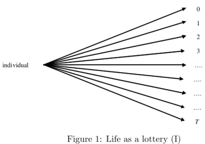
Figure 1 illustrates the lottery of life faced by a representative individual who facesT + 1possible scenarios regarding the duration of his life. Each scenario is characterized by a distinct duration of life. Life expectancy is computed by adding all possible durations of life, each of these being weighted by the probability of occurrence of each duration of life.
Durations of (remaining) life
0 1 2 3
individual … .
… .
… . .…
T
Figure 1: Life as a lottery (I)
If one denotes by pix the probability of a (remaining) life of durationxfor a personi, the mathematical expectation of the duration of (remaining) life for a personi, denoted byE(Li), can be written as:
E(Li) = XT x=0
pix x (1)
The probability of a life of durationxperiods for personican be written as:
pix=
xY1 s=0
(1 dis)dix (2)
where dis is the probability of death at age s for person i, conditionally on survival until ages. Substituting forpixin equation (1) allows us to rewrite life expectancyE(Li)as:
E(Li) =
TX1 x=0
Six+1 (3)
whereSix Yx 1
s=0(1 dis)is the unconditional probability of survival until age xfor personi. Life expectancy can be interpreted as a measure of the surface under the survival curve (which plotsSixas a function of x).2
There exist several types of life expectancy. Period life expectancies rely on age-speci…c probabilities of death prevailing at a particular period (usually one year). On the contrary, cohort life expectancy rely on age-speci…c probabilities of death prevailing during the entire life of a cohort. Period life expectancy is the most widely used because it can be computed year after year without having to wait for the death of all members of a given cohort.
At this stage, it is important to underline a key feature of period life ex- pectancy statistics. These measure the expected duration of life for some hypo- thetical "average" person. In reality, the actual duration of life may depend on lots of factors such as, among other things, the genetic background, lifestyles (sleeping patterns, physical activity, etc.), consumption patterns (smoking, drink- ing, etc.), risk-taking behaviors, preventive behaviors, environmental quality, etc. Period life expectancy statistics only provide some global picture of the survival conditions prevailing on average in a given population.
The major virtue of life expectancy indicators consists in their capacity to synthesize the prevailing survival conditions in one single number. However, life expectancies re‡ect only a single source of risk in human societies: the risk about one’sown survival. Besides that individual longevity risk, humans face many other sources of risk concerning, in particular, the survival of the persons they care about (spouse, children, parents, friends, etc.). The next subsection proposes an indicator taking that alternative source of risk into account.
2.2 Joint life expectancy
Recent empirical studies, such as Blanch‡ower and Oswald (2004), suggest that individuals care a lot about the survival of their spouse. The regressions carried
2As usual, we assumeSi0 = 1. Note that expression (3) presupposes that a person dying during a year dies at the beginning of that year. Alternatively, if one supposes that a person dying during a year dies, on average, in the middle of that year, (3) becomes:
E(Li) =
TX1
x=0
Six+1+ 0:5
out by those authors show that an amount of not less than $100,000 per year is necessary to compensate someone for widowhood. Such a large compensation reveals that individuals care not only about their own survival, but, also, about the survival of other persons.
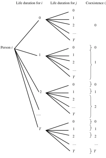
Once individuals have a strong concern for others’ survival, the represen- tation of life as a lottery in Figure 1 becomes incomplete. Actually, for each scenario concerning one’s survival, there exist lots of possible scenarios regarding the survival of other persons. For instance, it is not the same, for an individual, to survive until age 85 with his spouse, or to survive until age 85 while becoming a widow at the age of 70. Hence the representation of life as a lottery must be modi…ed, in such a way as to account for the various scenarios regarding others’
survival. To illustrate this, Figure 2 shows the lottery of life faced by a repre- sentative individualiwho cares not only about his own survival, but also about the survival of another individualj. That alternative representation treats life as a double lottery: for any possible duration of life for person i, there exist various possible durations of life for personj.3
We can, for each scenario in Figure 2, compute the duration of coexistence between the two individuals. The duration of coexistence for a particular sce- nario of life equals theminimum of the durations of life for the two individuals.
One can regard that duration of coexistence of two individuals as the duration of life for the group of two persons, provided a group disappears as soon as one of its members dies.
Once durations of coexistence are computed under each scenario of the dou- ble lottery, we can compute the mathematical expectation of the duration of coexistence. For that purpose, we aggregate all possible durations of coexis- tence for the two individuals, and we weight each of these by the probability of occurrence of that scenario. The outcome of that calculation consists of the periodjoint life expectancyof individualsiandj. This is the mathematical ex- pectation of the duration of their coexistence, or the average duration of life for that group, conditionally on the survival conditions prevailing during a period.
To illustrate this, let us take for instance two personsiandjof age 25. Each scenario of the lottery involves one duration of remaining life for personiand one duration of remaining life for personj. For each scenario of the lottery, one can compute the duration of remaining coexistence. This is equal to the minimum of the durations of remaining life for the two persons. If, for instance, both persons die at age 28, the remaining coexistence time equalsminf28 25;28 25g= 3 years. If, on the contrary, personi dies at age 45, but personj dies at age 42, the duration of remaining coexistence equalsminf45 25;42 25g= 17years.
Then, once the duration of remaining coexistence is computed for each scenario of the lottery, we can use the probabilities of occurrence of each scenario to calculate the mathematical expectation of the duration of remaining coexistence, that is, the joint life expectancy of individualsiandj (of current age 25).4
3Note that we restrict ourselves here to a double lottery, in which one person cares about his survival and about the survival of another person. But in the real world individuals may care about the survival of more than one other person, implying a more complex lottery.
4Similar calculations could be carried out for other groups of di¤erent size, including per-
Life duration fori Life duration forj Coexistence (i,j) 0
0 1
2 0
… T
Personi 0 0
1 1
2 1
… T
0 0
2 1 1
2
… 2
… . T
0 0
T 1 1
2 2
… …
T T
Figure 2: Life as a lottery (II)
More formally, if one denotes bypijx the probability of (remaining) coexis- tence of durationxfor two personsi andj, the joint life expectancy for those two persons, denoted byE(Lij), can be written as:5
E(Lij) = XT x=0
pijx x (4)
pijx depends on the survival conditions faced by persons i and j, and on how those survival conditions are related to each other. Alternatively, one can rewrite
sons of unequal ages.
5While that formula concerns the coexistence of two persons, joint life expectancies can also be de…ned for a larger number of individuals.
the joint life expectancy as the surface under the joint survival curve (which plots Sijxas a function ofx):
E(Lij) =
TX1 x=0
Sijx+1 (5)
where Sijx+1 is the unconditional probability of joint survival until x periods from now, for personsiandj. Sijx+1is the probability that both personsiand j are still alivexperiods from now.
As for period (single) life expectancies, period joint life expectancies do not, in general, coincide with the actual duration of coexistence for some individuals in reality. It consists, here again, of a statistical object, which measures some aspect of the survival conditions prevailing at a particular period. Period joint life expectancy statistics measure the expected duration of a group of individu- als, given the average survival conditions prevailing at a given period.6 It tells us, for instance, how many years two persons can expect, given the prevailing survival conditions, to coexist. In real life, coexistence may vary signi…cantly across groups, depending on the characteristics of each group. Hence, what joint life expectancy statistics give us is a global picture of the average joint survival perspectives at some period, in the same way as single life expectancies give us a global picture of survival perspectives at the individual level.
It is also important to stress that the joint life expectancy only measures
"coexistence" in a particular sense: it measures "coexistence" only from the perspective of joint survival. If, alternatively, one de…ned "coexistence" as the quantity of time lived together by two persons in the same spatial neighborhood, then there would exist many other factors than joint survival conditions that would also a¤ect the actual amount of so-de…ned “coexistence”. To illustrate this, take, for instance, the case of a couple. The number of life-years shared by the two members of a couple depends on lots of factors, and not only on the prevailing joint survival conditions. Actually, how long two members of a couple live together depends on the age at marriage, the divorce rates, profes- sional mobility, etc. Similarly, the so-de…ned "coexistence" between parents and children depends on many other things than joint survival conditions, such as the living arrangements, the duration of education degrees, the age at marriage, the unemployment rate for young people, etc.
Joint life expectancy statistics measure coexistence time in a di¤erent sense:
they measure how many years two individuals can expect to remain both alive, conditionally on the prevailing average survival conditions. Those measures do not tell us whether those individuals will live in the same house or not, will divorce or not, etc. All those aspects, which contribute to determine "coexis- tence" in the sense de…ned above, are not captured by the joint life expectancy, which focuses only on joint survival, independently from the circumstances un- der which this joint survival will take place. Similarly, single life expectancy statistics do not tell us whether the expected lifetime of an individual will be
6Alternatively, one may compute cohort joint life expectancies, on the basis of the survival conditions faced within a given cohort.
enjoyed under some particular circumstances, but only how many years one can expect to live. Thus, our joint life expectancy statistics only capture the pure joint survival component of the broad idea of "coexistence".
Having clari…ed the sense in which joint life expectancies measure the coex- istence phenomenon, let us now focus on the relationship between the survival probability of a group and the survival probabilities of its members. The joint survival probability for two individualsiandj Sijx+1 (i.e. the probability that both individuals i and j are still alive x periods from now) depends on the survival conditions faced by each individual separately, that is, survival proba- bilitiesSix+1 and Sjx+1. But the relationship between the joint survival prob- ability and individual survival probabilities may take various forms, depending on whether individual mortality risks are dependent or not, and, if so, on the sign (positive or negative) and extent of the dependence.
Positive dependence of individual mortality risks occurs when the premature death for a member of the group raises the probability of premature death for another member of the group. On the contrary, negative dependence prevails when the happening of premature death for a group member reduces the proba- bility of premature death for another member of the group. In those two cases, the relation between joint survival and individual survival is quite complex, and requires speci…c conceptual tools for the modelling of risk dependence.7
Besides those cases, there exists another case: the case ofindependentmor- tality risks. When mortality risks are independent, the duration of life for an individual i is una¤ected by the duration of life for an individual j. Hence, given that the survival chances of a person do not a¤ect the survival chances of any other person in that case, the joint survival probabilitySijx+1 is equal to the product of the probability that individualiis still alivexperiods from now times the probability that individualj is still alivexperiods from now:
Sijx+1=Six+1 Sjx+1 (6)
Hence, in that case, the joint life expectancy takes the form:
E(Lij) =
TX1 x=0
(Six+1 Sjx+1) (7)
Thus, when individual mortality risks are independent, the mathematical expec- tation of the coexistence time between two personsiandjis a sum of products of unconditional survival probabilities until di¤erent ages for those two persons.
Assuming that individual mortality risks are independent tends to simplify the analysis of coexistence. This explains why this assumption was made in some demographic studies of joint survival, as in Le Bras (1973 p. 11). Note, however, that this constitutes a signi…cant simpli…cation: in the real world, mortality risks faced by related individuals can be, to some extent, dependent, so that the joint survival probability is not equal to the product of individual survival
7Section 5 is dedicated to the measurement and valuation of coexistence gains when mor- tality risks are dependent.
probabilities, but takes a more complex form. Hence, when developing our empirical application, we will, in a …rst stage, consider the case of independent individual mortality risks as a …rst approximation (Section 4). Then, in Section 5, we will relax that assumption and introduce risk dependence.
3 Valuing coexistence time
In order to measure the value of coexistence time, we will, in the rest of this paper, rely on equivalent consumption measures, in line with the equivalent income approach. That method, which has become increasingly used in the literature aimed at valuing gains in life expectancy over time, is presented in Section 3.1. Section 3.2 extends it to the valuation of gains in coexistence time.
3.1 An equivalent consumption approach
A major di¢ culty raised by the inclusion of life-years in indicators of economic performance consists in the selection of adequate weights to represent the con- tribution of longevity gains relative to other determinants of well-being. This weighting problem arises because living standards are multidimensional. The equivalent income/consumption approach deals with the weighting problem by starting from (representative) preferences on hypothetical situations de…ned in terms of all dimensions of well-being under study. Those preferences are then used to construct an equivalent income/consumption aimed at measuring, in monetary terms, the well-being associated to some particular living condi- tions. The equivalent income/consumption is de…ned as the hypothetical in- come/consumption such that, if combined with reference levels for the other dimensions of well-being under study, it would bring the same well-being level as under the current income/consumption and the current living conditions.
In the context of the valuation of longevity gains, one can include longevity gains in a monetary measure of welfare by de…ning a constant consumption pro…le equivalent, that would, by construction, make a representative agent in- di¤erent between, on the one hand, his current situation (with current constant consumption pro…le and life expectancy), and, on the other hand, a hypotheti- cal situation with the equivalent consumption pro…le and the life expectancy of reference (usually the one prevailing at a base year).
Denoting by U(ci;Si) the utility function representing individual i’s pref- erences over lotteries of life de…ned as a pair (ci;Si), where ci is a vector of dimensionT+ 1, whose entries consist of constant consumption levels at each (potential) period of life, whileSi is a vector of dimensionT+ 1, whose entries consist of unconditional survival probabilities to the di¤erent ages of life, one can de…ne the constant consumption pro…le equivalent^ci in the following way:
U(ci;Si) =U ^ci;Si (8) whereSi represents the reference survival conditions.
The constant consumption pro…le equivalent ^ci captures, by construction, the welfare gains associated with an improvement in survival conditions. To see this, note …rst that if the actual survival conditions are equal to the reference survival conditions (i.e. ifSi =Si), then the current consumption pro…le and the equivalent consumption pro…les are equal: ^ci =ci. However, if the actual survival conditions are better than the reference survival conditions, i.e. if Si Si, we haveci ^ci, re‡ecting the improvement in the quality of life.
Assuming that (i) individual preferences satisfy the expected utility hypoth- esis (i.e. preferences on lotteries are represented by a weighted sum of utilities associated to the scenarios of those lotteries, with weights corresponding to the probability of occurrence of each scenario), (ii) lifetime welfare is a discounted sum of temporal welfare levels (with some constant pure time preference factor
), (iii) temporal welfare takes the form c
1 i
1 + , we can represent individual i’s preferences by:
U(ci;Si) =
TX1 s=0
sSis+1
c1i
1 +
!
(9) From which we can write the equivalent consumption ‡owc^i (i.e. the entry of the constant equivalent pro…le^ci) as satisfying the following equality:
TX1 s=0
sSis+1 c1i
1 +
!
=
TX1 s=0
sSis+1 ^c1i
1 +
!
(10) From which it follows that the equivalent consumption ‡owc^i is:
^ ci=
8>
<
>:(1 ) 2 64
0 B@
XT 1 s=0
sSis+1 c1i
1 +
XT 1 s=0
sSis+1
1 CA
3 75
9>
=
>;
1 1
(11)
The equivalent consumption ‡ow^ci is such that, if enjoyed every year while facing the survival conditions of reference, this would make the representative agent indi¤erent between that hypothetical situation and his current situation (with current consumption pro…le and survival probabilities). The equivalent consumption ‡ow allows us to incorporate, within an extended monetary mea- sure of economic performance, variations in survival conditions with respect to reference survival conditions. Expression (11) shows how preferences, through the parameters , and , a¤ect the shape of the constant equivalent con- sumption level^ci. The gap between the actual and the equivalent consumption levels depends on the di¤erential between the existing survival conditions and the survival conditions of reference.
The monerary equivalent method was used, with several amendments, in Williamson (1984), Crafts (1997), Costa and Steckel (1997), Sandberg and Steckel (1997), Nordhaus (2003), Becker et al (2005), Murphy and Topel (2006), Hall and Jones (2007) and Fleurbaey and Gaulier (2009). Those studies high- lighted that the measurement of economic performance over time is strongly
a¤ected by the inclusion of variations in survival conditions. In the following, we propose to extend that approach to the inclusion of variations in joint sur- vival conditions.
3.2 Equivalent consumption under coexistence concerns
When an individual cares about coexistence withM >0other individuals, his utility function depends not only on his consumption and on his own survival chances, but also on how long he expects to coexist with each of those M individuals. This latter determinant of his well-being can be measured by the joint life expectancies with those persons. Since joint life expectancies depend on the survival conditions faced by each of those persons (because Sijx+1 is a function of Six+1 and Sjx+1), the well-being of our representative individual depends now on the survival conditions faced by theM persons of interest.8
In that context, we can rede…ne the constant consumption pro…le equivalent, as the hypothetical constant consumption pro…le that would, by construction, make a representative agent indi¤erent between, on the one hand, his current situation, with his current consumption and the current survival conditions (both for himself and for the M persons he cares about), and, on the other hand, a hypothetical situation with the constant equivalent consumption pro…le and the survival conditions of reference (both for himself and theM persons).
If one denotes byU~(ci;Si;S1; :::;SM)the utility function of individualithat represents his preferences over lotteries involving di¤erent durations of life for him as well as for the M other persons, the constant equivalent consumption pro…le^ci now satis…es the condition:
U~(ci;Si;S1; :::;SM) = ~U ^ci;Si;S1; :::;SM (12) whereSi;S1; :::;SM are the unconditional survival probabilities of reference for personsiand for the M persons. Under that formulation, the constant equiv- alent consumption pro…le captures not only the variations, with respect to the survival conditions of reference, in the survival conditions faced by individuali, but also the variations in the survival conditions faced by theM other persons.
Assuming that individuali’s preferences satisfy conditions (i) and (ii), and replacing (iii) by assumption (iv), according to which temporal welfare equals
c1i
1 + +XN
q=1 qin case of coexistence withNpersons (out of theM persons he cares about), the utility functionU~(ci;Si;S1; :::;SM)can be written as:
U~(ci;Si;S1; :::;SM) =
TX1 s=0
sSis+1 c1i
1 +
! +
XM q=1
q TX1
s=0
sSiqs+1 (13)
where q is the intensity of individual i’s coexistence concerns with person q.
The function U~(ci;Si;S1; :::;SM) can be decomposed in two components: on
8The form of the relation between the probabilities of joint survival (and, hence, the joint life expectancy) and individual survival probabilities may vary, depending on how dependent individual survival processes are. See Section 5 on this.
the one hand, the expected welfare from consumption of goods and services (…rst sum of terms), which depends on individuali’s survival probabilities; on the other hand, the expected welfare from coexistence with the M persons of interest (second sum of terms), which depends on the joint life expectancy of individualiwith each of those persons of interest.9
The additive structure of U~(ci;Si;S1; :::;SM)implies that the welfare gain from coexisting with one person isindependentfrom the welfare gain from coex- isting with other persons. Note that, in the real world, it may be the case that the welfare derived from coexistence with a person depends on the presence of some other person. However, there is, in general, no obvious way to relate the welfare gains from coexistence with di¤erent persons. In that context, assuming an additive structure is a plausible …rst-order approximation.
On the basis ofU~(ci;Si;S1; :::;SM), we can write the equivalent consump- tion ‡owc~i (i.e. the entry of the constant equivalent pro…le^ci) as satisfying:
TX1 s=0
sSis+1 c1i
1 +
! +
XM q=1
q TX1 s=0
sSiqs+1
=
TX1 s=0
sSis+1 ~c1i
1 +
! +
XM q=1
q TX1 s=0
sSiqs+1 (14)
Isolating the equivalent consumption ‡ow~ci, one obtains:
~ ci =
8>
<
>:(1 ) 2 64
0 B@
XT 1 s=0
sSis+1 c1i
1 + +XM
q=1 q q
XT 1 s=0
sSis+1
1 CA
3 75
9>
=
>;
1 1
(15) where q XT 1
s=0
sSiqs+1 XT 1 s=0
sSiqs+1.
As in the baseline model,~cidepends on individuali’s survival chances, and on preference parameters , and . However, under coexistence concerns,
~
ci depends also on the joint survival chances of individual i with each of the M persons of interest, and on the preference parameters q, which capture the welfare gains from coexistence with each of those persons. As a consequence,
~
ci captures not only the variations in life expectancy for personi, but also the gains in joint life expectancy with the persons of interest.
9The utility function is assumed to exhibit self-oriented coexistence concerns: according to that function, individuals care about the survival of other persons only for themselves, without caring about the well-being of those other persons. It should be stressed here that this utility function does not constitute the only way to represent coexistence concerns. As an alternative to self-oriented coexistence concerns, we could have represented coexistence concerns by means of a utility function exhibiting altruism (individuals would be interested in the well-being of others, and, hence, in the survival of others).
4 An illustration with French data (1820-2010)
Let us now illustrate the above discussions in the light of the example of France (1820-2010). For that purpose, we will proceed in two stages. Section 4.1 presents joint life expectancy statistics for France, and discusses the evolution of the generational overlap over time. Section 4.2 proposes to quantify the contribution of improved joint survival conditions to living standards, under di¤erent scenarios regarding the structure of coexistence concerns.
Throughout this section, we will …rst focus, for the sake of simplicity, on the case where individual mortality risks are independent, so that the joint life expectancies can be written as a sum of products of individual unconditional survival probabilities. Then, Section 5 will examine the robustness of our results to introducing mortality risk dependence by means of the copula approach.
4.1 Joint life expectancies
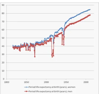
The demographic data that we use are the lifetables from theHuman Mortality Database for France (1816-2010).10 In order to give a general view of the evo- lution of survival conditions over that period, Figure 3 presents the patterns of life expectancy at birth for men and women over that period. Life expectancy has strongly grown: the expected duration of life was, in 1816, about 39 years for men and about 41 years for women, it is nowadays about 78 years for men and 85 years for women. The three drops coincide with the French Commune (1871), the First and the Second World War.
Given the observed improvement of survival conditions, one expects that the duration of coexistence between individuals must have increased too. However, without any further calculations, it is hard to know to what extent coexistence time has grown over time. Actually, as we will show below, the precise extent to which coexistence has grown depends on the particular age of the individuals whose coexistence is considered.
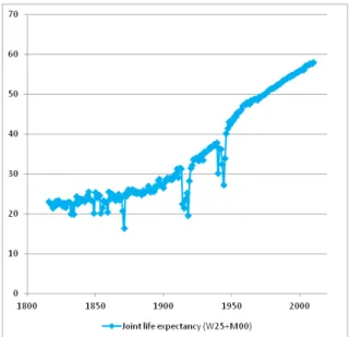
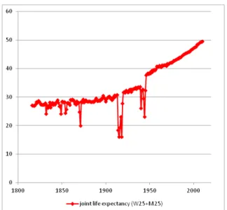
Let us take, as a …rst case, the coexistence of a man and a woman of age 25 years in France (Figure 4). During the 19th century, the joint life expectancy of a man and a woman of age 25 was relatively stable, and equal to about 28 years. However, there has been a strong growth in coexistence time during the 20th century. In 2010, a man and a woman of age 25 can expect to coexist about half a century. Note also, still on Figure 4, that the expected coexistence has decreased strongly during the French Commune, the First and the Second World Wars. If one interprets the pair of a man and a woman as a couple, those drops show that, in times of con‡ict, a signi…cant part of the population falls in widowhood, implying a decline in the average coexistence time for couples.11
1 0Sources: The Human Mortality Database (2013), University of California, Berkeley (U.S.), Max Planck Institute for Demographic Research (Germany). Available online at:
http://www.mortality.org. Note that Section 4.1 presents demographic data over 1816-2010, whereas our income data only cover the period 1820-2010. Hence, demographic data for years 1816-1819 will not be used when computing consumption equivalents (Section 4.2).
1 1Note that, if one carries out the same computation exercise for a pair composed of a man and a woman of age 50 years, one …nds a similar pattern: stagnation of the joint life
Figure 3: (Period) life expectancy at birth in France, 1816-2010, women and men
When interpreting Figure 4, it should be stressed that joint life expectancies quantify coexistence only from the perspective of joint survival. Those measures quantify the expected time during which both a male and a female of some ages will remain alive. But there is no concern here for divorce, living arrangements, or other factors a¤ecting coexistence in a broader sense.
Joint life expectancies can also be used to measure the duration of coex- istence for persons who belong to di¤erent generations, that is, the overlap between generations. Figure 5 shows the joint life expectancy of a woman of age 25 with a newborn boy over 1816-2010. The expected duration of coex- istence for those persons has been multiplied by a factor (almost) equal to 3, from about 22 years in 1816 to about 60 years in 2010. The rise in the joint life expectancy is here larger than the rise in the life expectancy of the two per- sons taken separately. Actually, life expectancy has, over that period, doubled (approximately), whereas the joint life expectancy was multiplied by 3. If one interprets Figure 5 as showing the expected duration of coexistence for a young mother with her newborn boy, it follows that the average size of the overlap between two successive generations has grown strongly during the 20th century.
expectancy during the 19th century, and strong growth during the second part of the 20th century. While a man and a woman of age 50 could expect to coexist about 15 years in the 19th century, their expected duration of coexistence is now equal to 28 years.
Figure 4: (Period) joint life expectancy for a woman and a man of age 25, France (1816-2010)
Figure 5: (Period) joint life expectancy for a woman of age 25 and a newborn boy, France
(1816-2010)
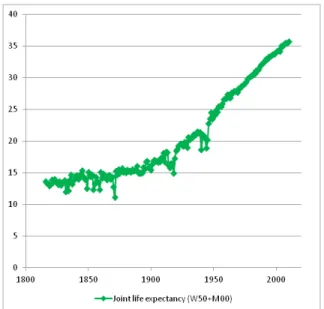
In a similar vain, Figure 6 shows the joint life expectancy for a woman of age 50 with a newborn boy. Whereas coexistence between them was about 15 years
during the 19th century, this is today above 35 years. If one assumes generations of 25 years, that joint life expectancy can be interpreted as the average size of the overlap between two generations separated by an intermediate generation.
Coexistence with a grandmother lasted, on average, less than 15 years during the 19th century. Nowadays, it lasts more than 35 years.
Note, here again, that joint life expectancy measures coexistence only in a particular sense, that is, from the perspective of joint survival. Many other factors can a¤ect the size of the overlap between generations. For instance, the recent tendency towards the postponement of births starting in the 1970s (see Gustafsson 2001) may tend to reduce, to some extent, the contribution of the rise in joint life expectancies to the overlap between generations. However, if we consider the overlap of two successive generations (Figure 5), the postponement of births a¤ects the overlap in a way that is, over the entire period considered, likely to be far less sizeable than the impact of improved joint survival conditions.
It is only for the overlap of non successive generations, as on Figure 6, that the postponement of births could have a more signi…cant impact on the generational overlap (in case of repeated postponement of births at each generation).
Figure 6: (Period) joint life expectancy for a woman of age 50 and a newborn boy, France
(1816-2010)
An alternative way to measure the evolution of coexistence time consists of joint survival curves. Those curves are the equivalent, for the measure of coexistence time, of standard survival curves focusing on the lifetime of a single individual. A joint survival curve indicates the probability that a group of
individuals of some particular age and gender achieves a particular duration of existence, conditionally on age-speci…c probabilities of survival.
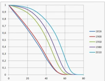
Figure 7: Joint survival curves (period) for a man and a woman aged 25.
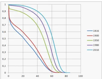
Figure 8: Joint survival curves (period) for a woman aged 25 and a newborn boy.
As an illustration, Figure 7 shows the evolution of joint survival curves in the case of groups composed of a man and a woman of age 25. On the basis of age-speci…c mortality rates prevailing in 1816, only 23.5 % of pairs composed of a man and a woman of age 25 would still be complete 40 years later, whereas 76.5 % of those pairs would have, during the next 40 years, su¤ered from the
death of at least one of their members. But if we focus on the survival conditions prevailing in 2010, the proportion of pairs still complete 40 years later is equal to 77.5 %, that is, more than three times larger than in 1816. The evolution of coexistence time over the last two centuries appears even stronger once one focuses on the proportion of pairs of individuals still complete after a period of 60 years. That proportion has grown from 2 out of 1000 on the basis of 1816 survival conditions, to 245 out of 1000 on the basis of 2010 survival conditions.
In a similar vein, Figure 8 shows the evolution of joint survival curves for a pair composed of a woman of age 25 and a new-born boy. Here again, the gains in terms of coexistence time are substantial. Whereas only 25.5 % of those pairs remained complete 40 years later on the basis of 1816 survival conditions, that proportion grew to 33 % in 1900, to 69 % in 1950, and reaches 90 % in 2010.
If one interprets those pairs as pairs composed of a mother and her child, the latter number means that, conditionally on age-speci…c probabilities of death prevailing in 2010, 90 % of children will coexist at least 40 years with their mother. That …gure is about 4 times larger than in 1816.
Note that Figure 8 shows the evolution of joint survival under a given, …xed age gap between the woman and the boy, equal to 25 years. This …xed age gap constitutes a simpli…cation of reality. In particular, the recent tendency towards the postponement of births has increased the average age gap between mothers and sons (Gustafsson 2001). However, this trend is recent in comparison with the long-lasting improvement in survival conditions. Moreover, the rise in the age gap does not su¢ ce to fully counterbalance the large gains achieved in terms of joint survival.
4.2 Equivalent consumptions
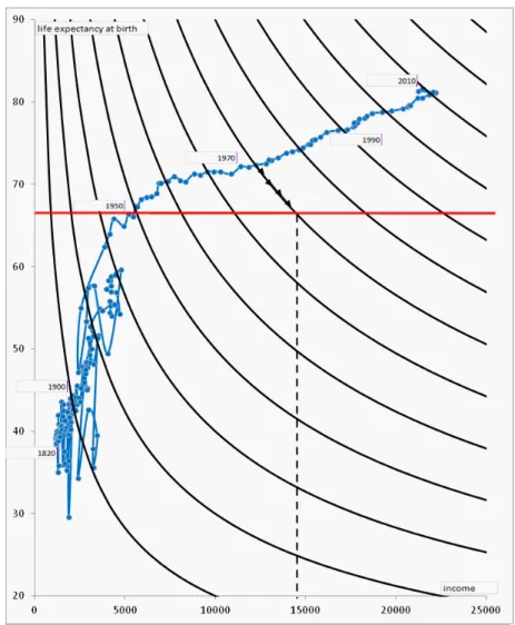
In this section, we calculate the value of coexistence years by using the method of consumption equivalents that was presented in Section 3. That method can hardly be illustrated geometrically, since the number of dimensions under study (i.e. consumption per year and survival conditions per year) is too large. How- ever, for the sake of illustration, we can represent geometrically the construction of monetary equivalents by focusing on a simple two-dimensional case, involving only income and life expectancy. That case is illustrated on Figure 9, with the example of France (1820-2010).12 Figure 9 shows the evolution of France in the (income, life expectancy) space. Provided one draws an indi¤erence map in that space, it is possible to compute an equivalent income for each year, under some particular baseline survival conditions.13
If, for instance, one chooses the life expectancy prevailing in 1950 as a refer- ence, one can, for each year under study, compute the hypothetical income level
1 2The income …gures are GDP per capita expressed in International Geary-Khamis dol- lars (1990). Sources: The Maddison Project: http://www.ggdc.net/maddison/maddison- project/home.htm. Life expectancy …gures come from the Human Mortality Database (2013).
1 3The indi¤erence map on Figure 9 is drawn in an arbitrary way. The next subsection explores the construction of a more realistic indi¤erence map on the basis of the empirical literature on money/risk and risk/risk trade-o¤s.
that would maintain the representative agent on the same indi¤erence curve, while facing the 1950 survival conditions.14 Figure 9 illustrates the computa- tion of the equivalent income for year 1972. The equivalent income is obtained by moving along the indi¤erence curve passing through the 1972 point, until one reaches the 1950 life expectancy level.
Figure 9: Construction of the equivalent income for year 1972 in France.
This section, which computes constant consumption pro…le equivalents, car- ries out the same kind of computation of monetary equivalents, but in a di¤erent
1 4The reference survival conditions - here the ones prevailing in 1950 - were chosen ar- bitrarily. A similar construction could be carried out under alternative reference survival conditions.
space, including more dimensions (consumption per year and survival conditions per year), as presented in Section 3. The major di¢ culty raised by the equivalent consumption approach consists of drawing the indi¤erence map in the space un- der study. Obviously, given that both consumptions and survival conditions are in general desirable goods, indi¤erence curves must be decreasing. Moreover, one expects also that very short lives with high consumptions and very long lives with low consumptions must be dominated, in welfare terms, by lives with intermediate duration and intermediate consumptions. As a consequence, it is also reasonable to expect that indi¤erence curves are convex. Having stressed this, one needs additional information to be able to draw the indi¤erence map.
The next subsection shows how one can draw such indi¤erence maps on the basis of empirical studies on money-risks and risks-risks trade-o¤s.
4.2.1 Calibration of preference parameters
In our model, the knowledge of preference parameters , , and K would allow us to draw an indi¤erence map in a space including, as dimensions, con- sumptions at di¤erent ages as well as individual and joint survival probabilities.
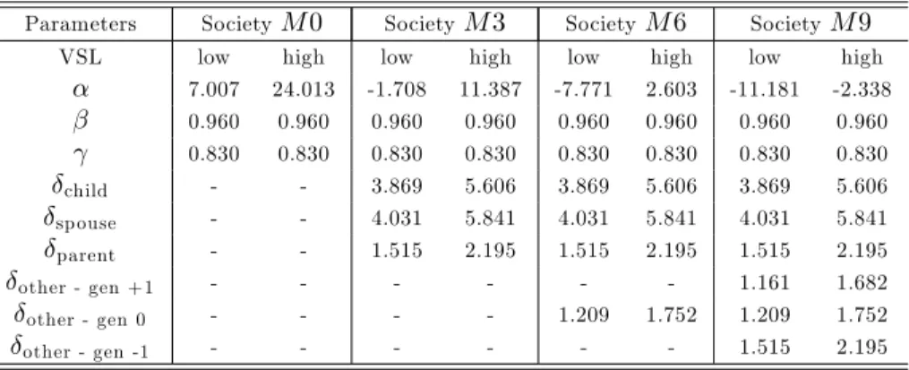
For the sake of presentation, we will focus on the case of a representative agent of age 25.15 When considering the calibration of preferences, it is clear that there exists a strong heterogeneity in real life, concerning both the strength and direction of coexistence concerns. We will consider here four distinct cali- brations, each of these corresponding to a more or less dense network of welfare interdependencies (i.e. a more or less high numberM of persons of interest):
1. CaseM0: Absence of welfare interdependencies (M = 0) 2. CaseM3: Weak interdependencies (M = 3)
3. CaseM6: Strong interdependencies (M = 6) 4. CaseM9: Extended interdependencies (M = 9)
CaseM0, where individuals only care about their own survival, is implausi- ble, but will be used as a benchmark. Regarding casesM3 to M9, we assume that social interdependencies are uniformly distributed in terms of generations.
In other words, the persons whose survival matters for an individual of age 25 will be supposed to be of ages 0, 25 and 50 years in equal proportions.16
The calibration of parameters and can be based on the existing literature.
The parameter , which re‡ects pure time preferences, takes in general a value
1 5The reason why we do not consider lower ages is that our consumption data do not cover ages inferior to 25 years (see the Appendix).
1 6In the case of societyM3, it is assumed that the representative individual cares about the survival of a spouse, of a child and of a parent. In the case of societyM6, it is assumed that the representative agent cares about the survival of one spouse, of two parents and of two children. Finally, in the case of societyM9, it is assumed that the representative individual cares about the survial of one spouse, two parents and two children, as well as of one person of his generation, one person of the previous generation and one person of the next generation.
that is consistent with a quarterly discount factor equal to 0.99 (see de la Croix and Michel 2002). In our model, where each period lasts one year, the adequate value of is equal to(0:99)4= 0:96. As far as the calibration of is concerned, empirical studies surveyed in Browning et al (1999) lead to values close to0:85.
Following Blundell et al (1994), we will use = 0:83.
Regarding the calibration of parameters and K, we will rely on the liter- ature on money/risk trade-o¤s. The literature on the value of a statistical life (VSL) - i.e. the shadow price of a reduction of the risk of death per unit of risk - is broad, and includes studies of two distinct types: revealed preferences studies (focusing on how individuals solve the money/risk trade-o¤ on existing markets) and stated preferences studies (asking to individuals their willingness to pay - WTP - or their willingness to accept - WTA - for small variations in the risk of death).17 Despite signi…cant variations across methods (the WTA being generally larger than the WTP for an equal variation of risk), VSL studies all showed that reductions of the risk of death are highly valued (see Aldy and Viscusi 2003). According to Miller (2000), the VSL amounts to between 120 and 180 times the GDP per capita. This indicates that individuals strongly value reductions in the risk of death, even though VSL estimates vary according to variables such as income, health status and age (see Cropper et al 2011).
Empirical estimates of the VSL can be used to calibrate parameters and
K. For that purpose, let us assume, as a …rst approximation, that individual mortality risks are independent.18 If one de…nes, like Jones-Lee (1991), the VSL as the average marginal rate of substitution between consumption and the risk of death within the population, the VSL can be written, in our model with homogeneous population, as:
@c0t
@dI0t U( )=U
=
@U( )
@dI0t
@U( )
@c0t
= 2 64
XT 1 i=0
iSIi+1t c1
i
1 +
(1 dI0t)
+XM K=1 K
XT 1 i=0
iSIKi+1t
(1 dI0t)
3 75
(1 dI0t)(c0t) (16) whereSIi+1t denotes the probability of survival for the representative agentI until periodi+1on the basis of mortality tables prevailing at timet,dI0tdenotes the probability of death in the …rst period for the representative individualI on the basis of mortality tables prevailing at timet, while SIKi+1tdenotes the probability of joint survival for the representative individualI with individual Kuntil periodi+ 1on the basis of mortality tables prevailing at timet.19
In the case M0, where there is no interest for coexistence (i.e. K = 0 for
1 7On revealed preferences studies, see the survey by Viscusi (1998). On stated preferences studies, see Johansson (1995). Stated preferences studies are sub ject to framing e¤ects (see Andersson et al 2013 for recent evidence of time framing e¤ects).
1 8The calibration of preference parameters under dependent mortality risks is examined in Section 5.
1 9Survival probabilities are taken from theHuman Mortality Database. For simplicity, we take survival probabilities for the total population (men and women).
allK), the above expression can be simpli…ed to:
@c0t
@dI0t U( )=U
=
@U( )
@dI0t
@U( )
@c0t
=
XT 1 i=0
iSIi+1t c1
i
1 +
(1 dI0t)
(1 dI0t)(c0t) (17) From that expression, it is possible, for empirical estimates of parameters and and for empirical estimates of the VSL, to extrapolate a value for preference parameter from mortality tables and consumption pro…les.20 To see this, note that isolating yields:
=
V SL (1 dI0t)(c0t) XT 1 i=0
iSIi+1t
(1 dI0t) c1i
XT 1 1 i=0
iSIi+1t
(1 dI0t)
(18)
According to Miller (2000), the VSL amounts to between 127 and 184 times the real GDP per capita, that is, between 2466928 and 3574132 euros (2000).
Substituting for those estimates in the above expression, as well as for = 0:96 and = 0:83, one obtains = 7:007 under the lower bound for VSL and
= 24:013 for the upper bound.21
Those values for presuppose the absence of coexistence concerns, i.e. K = 0 for all K. Once individuals are interested in other individuals’ survival (as in cases M3, M6 and M9), one needs to calibrate and K jointly. Such a calibration requires to know how individuals value the survival of others.
While studies measuring the value of variations inindividualsurvival prospects are numerous, the same is not true for studies measuring the value of variation in joint survival prospects. One exception is the study by Needleman (1976), which uses data on kidney transplant in order to identify "coe¢ cients of con- cerns", which are marginal rates of substitution between the risk of death for a given person and the risk of death for another person.22 Kidney transplant situations are most relevant for the valuation of coexistence gains, since these are cases where individuals must make a trade-o¤ between the survival of an- other person (the potential receiver) and their own survival. Hence Needleman’s estimated coe¢ cient of concerns based on kidney donations are most relevant for calibrating a lifecycle model with coexistence concerns.
Needleman’s estimated coe¢ cients of concern vary depending on the link between the potential donor and the potential receiver. Needleman found that the coe¢ cient of concern for a person and his spouse is equal to about 0.1. This means that, in order to increase the survival chances of his spouse, a person is willing to sacri…ce, in terms of his own survival chances, at most one tenth of that variation. When considering other links, coe¢ cients of concerns are even
2 0See the Appendix for data on consumption pro…les.
2 1Given that Miller’s study covers the period 1974-1999, we use, for the calibration, the average levels of the variables (consumptions, survival probabilities) over that period.
2 2Other studies on the interest of individuals for others’ survival include Jones-Lee (1991), Araya and Leon (2002) and Strand (2005).