[PENDING] Contribution à la planification de mouvement pour robots humanoïdes

HAL Id: tel-00446757

https://tel.archives-ouvertes.fr/tel-00446757

Submitted on 13 Jan 2010

HAL is a multi-disciplinary open access archive for the deposit and dissemination of sci- entific research documents, whether they are pub- lished or not. The documents may come from teaching and research institutions in France or abroad, or from public or private research centers.

L’archive ouverte pluridisciplinaire HAL, est destinée au dépôt et à la diffusion de documents scientifiques de niveau recherche, publiés ou non, émanant des établissements d’enseignement et de recherche français ou étrangers, des laboratoires publics ou privés.

Contribution à la planification de mouvement pour robots humanoïdes

Oussama Kanoun

To cite this version:

Oussama Kanoun. Contribution à la planification de mouvement pour robots humanoïdes. Automatic.

Université Paul Sabatier - Toulouse III, 2009. English. �NNT : �. �tel-00446757�

THÈSE THÈSE

En vue de l'obtention du

DOCTORAT DE L’UNIVERSITÉ DE TOULOUSE DOCTORAT DE L’UNIVERSITÉ DE TOULOUSE

Délivré par l'Université Toulouse III - Paul Sabatier Discipline ou spécialité : Automatique

JURY

Oussama Khatib Rapporteur Philippe Bidaud Rapporteur Jean-Paul Laumond Examinateur

Etienne Ferré Examinateur Pier-Giorgio Zanone Examinateur

Florent Lamiraux Examinateur

Ecole doctorale : Systèmes (EDSYS)

Unité de recherche : CNRS - Laboratoire d'Analyse et d'Architecture des Systèmes Directeur(s) de Thèse : Jean-Paul Laumond

Rapporteurs : Oussama Khatib (Stanford University) et Philippe Bidaud (UPMC) Présentée et soutenue par

Oussama Kanoun

Le

26 octobre 2009

Titre :

Contribution à la planification de mouvement pour robots humanoïdes

To Neila, Foued and Karim

Acknowledgements

This work has been part of the research project Zeuxis for which we gratefully acknowledge a sponsorship from

I owe the fantastic experience I had during my thesis to people of great caliber. First, I realize how big a chance it was to work under the supervision of Dr.Jean-Paul Laumond whom I thank for his guidance and accommodating management. I had the chance to work with Dr.Florent Lamiraux whose scientific advice was a constant reason behind successes. The fact that I could easily concentrate on my thesis topic was largely due to the support of Dr.Anthony Mallet, author of a great robotics software architecture.

The teamwork we put forward to achieve vision-guided grasp for HRP-2 was one of the best moments of this thesis. I would like to thank Dr.Eiichi Yoshida who directed me to a lot of essential material and provided friendly support and counsel. I also had the chance to collaborate with Dr.Pierre-Brice Wieber from whom I learnt a lot.

Like the legendary singer said, I get by with a little help from my friends. So thank you Anh, Claudia, Wael, Gustavo, Thierry, Brice, Ali, Mathieu, Seb, Carlos, Manish, Pancho, Diego, David, Layale, Thomas and Duong. Special thanks go to Zen-master Minh :). Special thanks to you Antoine and Muriel, for your constant friendship and fantastic meals :)! Grazie mille Soraya, J´erˆome, Virginie, Marrrie and Diarmait.

Big thanks fly to my adorable family in Tunis and Sfax and everywhere else in the world.

I owe and dedicate this achievement to my mother Neila, my father Foued and my brother Karim who

have always had infinite unconditional support, encouragement and trust. Thank you for your love, far

better than anything in this world.

Contents

1 Introduction 1

1.1 Problem statement . . . . 1

1.2 Related works and contributions . . . . 2

1.3 Outline of the thesis . . . . 4

1.4 Associated publications and software . . . . 5

2 Classical prioritized inverse kinematics 7

2.1 Definitions . . . . 7

2.2 Differential kinematics . . . . 8

2.3 Local extrema, or singularities . . . . 10

2.4 Prioritization . . . . 12

2.5 Handling inequality constraints . . . . 15

3 Generalizing priority to inequality tasks 19

3.1 Inequality task definition . . . . 19

3.2 Description of the approach . . . . 21

3.3 Mapping linear systems to optimization problems . . . . 21

3.3.1 System of linear equalities . . . . 22

3.3.2 System of linear inequalities . . . . 23

3.3.3 Mixed system of linear equalities and inequalities . . . . 24

3.4 Prioritizing linear systems . . . . 24

3.4.1 Formulation . . . . 24

3.4.2 Properties . . . . 25

3.4.3 Algorithms . . . . 25

3.4.4 Dealing with singularities . . . . 27

3.5 Conclusion . . . . 29

4 Illustration 31

4.1 A humanoid robot . . . . 31

4.2 Constraints and tasks . . . . 33

4.3 Prioritization . . . . 43

5

5 Dynamic walk and whole body motion 49

5.1 Dynamic walk generation . . . . 50

5.1.1 Dynamic constraints . . . . 50

5.1.2 A model approximation . . . . 51

5.1.3 An optimal controller . . . . 52

5.1.4 Merger with prioritized inverse kinematics . . . . 55

5.2 Experiments . . . . 57

6 Footsteps planning as an inverse kinematics problem 63

6.1 Principle of the approach . . . . 63

6.2 Construction of inverse kinematics problems . . . . 64

6.2.1 A single footstep . . . . 64

6.2.2 Several footsteps . . . . 67

6.3 Tuning the parameters . . . . 68

6.3.1 Number of footsteps . . . . 68

6.3.2 Starting footstep . . . . 70

6.4 Illustration . . . . 71

6.5 Conclusion . . . . 76

7 Integration 79

7.1 The full algorithm . . . . 79

7.2 Illustration . . . . 80

8 Conclusion 91

1

Introduction

1.1 Problem statement

Autonomous robots concretize a Perception-Planning-Action loop. Perception is the construction of a useful representation of the robot and its environment. This process relies on data produced by cameras, range sensors, force sensors, gyroscopes, etc. Actions designate the events that the robot can provoke such as signals (light, voice), motions (involving motors, pneumatics), etc. Planning is the process that maps the perception to actions. In this thesis, we will be exclusively focusing on planning problems for humanoid robots.

The planning component of a humanoid robot designed after the human form is a great challenge to roboticists. In front of a robot with a human shape walking and moving dexterously, anyone would rightfully expect a little intelligence in the package. Intelligence, for a machine, is the capacity to perform tasks normally requiring human intelligence (Oxford dictionary). All there seems to do to test this intelligence is to submit a task and compare the robot’s actions to one’s own. This is the principle of The Turing Test. The robot should use all the resources at its disposal and adopt a course of actions that a human would expect from his peers.

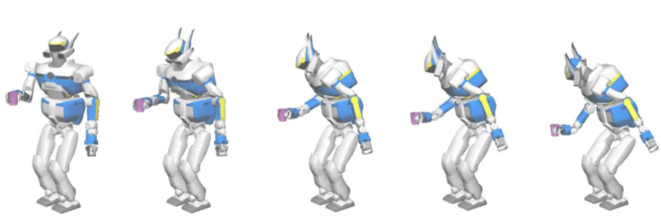
Intelligence can be perceived at very simple levels. For instance, to grasp a couple of cups standing close on a table, the human would probably use both hands simultaneously if possible. A humanoid robot with the same possibility taking a cup after the other may probably be dismissed from the closed circle of intelligent robots. Intelligence can be perceived on the level of the action itself: if the table happens to be a little low, instead of decomposing the action into leaning forward on the legs then stretching the arms to grasp the cups, all involved parts of the robot could move simultaneously to achieve the task.

1

In both examples, intelligence is reflected through the coordination of several resources to save time.

In the second example, the robot used its legs to help a manipulation. We might have little conscience of the motion of our lower bodies when performing such manipulation tasks. We may also have little conscience of the infinity of ways in which we could have solved the same problem. One important aspect of the intelligence of humanoid robots must therefore be a seamless exploitation of their rich and redundant mechanical structures.

Unlike humans who might indulge in walking for their pleasure or because it sustains their health, the humanoid robot should be motivated by a precise task for obvious energy-related considerations. How do we relate the steps that we make to the tasks that we perform with our hands or any other part of our bodies? Again, when we think of the number of solutions we realize that the robot must often choose from an infinity, which it still has to be aware of. Let us again consider the simple example of picking up an object, from the floor this time. We have not yet spoken of a level of intelligence to build a piece of furniture from a famous Swedish brand, we will merely ask the robot to collect the fallen assembly manual. The robot, nonetheless, faces various difficulties: where to stand to be able to perform the task?

The object is on the ground, therefore it will probably need to crouch, so how to take this posture into account for the motion plan? Is the task feasible at all given its body shape? We are hinting at a second seamless form of intelligence: the humanoid robot must decide if it needs to resort to locomotion in order to carry out a task and if so, find a suitable one.

In fact, most animals possess this level of intelligence, they flawlessly move to where an intended action could be fulfilled. The motion of legged forms on a terrain could roughly be seen as a monotonous translation and/or rotation to attain a remote objective. However, a fine adjustment occurs at the end of the locomotion so that the posture is adapted to the intended action. The complexity of actions and postures is much higher for bipeds than for four-legged animals, therefore any heuristic-based resolution of the task-driven locomotion problem is too restrictive.

The planning component of a humanoid robot must rigorously relate its tasks to its whole body and locomotion capabilities, otherwise even the simplest possible tasks could be failed. We aimed in our work at answering this requirement.

1.2 Related works and contributions

The two major components of this topic, whole body motion generation and locomotion planning, have been subject to an extensive research activity. Both subjects could be considered new in the overall young field of robotics. This thesis advances a new view for each subject.

In the context of robot motion control, a task is defined as a desired kinematic or dynamic property

in the robot (e.g position of hand, forces applied on manipulated object, direction of cameras, etc). For

robotic arms with a few degrees of freedom, we may find analytical formulas giving the unique control

satisfying a desired task. For highly-articulated structures like humanoid robots, the kinematic structure

is often redundant with respect to a task, offering an infinity of possible controls to choose from. One efficient way of solving the problem of control in redundancy is by identifying a task to the minimum of a convex cost function that can be reached using a numerical algorithm. If we wanted to take advantage of the redundancy of the system and assigned several tasks at a time, we could still resort to the same algorithm and minimize the sum of the cost functions associated with the tasks. However, if the tasks became conflicting, the numerical algorithm could lead to a robot state where none of them are satisfied.

To avoid such situations, it has been proposed to strictly prioritize tasks so that when such a conflict occurs, the algorithm should privilege the task with higher priority. Such a prioritization of a task A over a task B has been modeled in [Li´egeois 1977] as the control for task B within the set of controls satisfying task A. The framework was further developed in [Nakamura 1990] and extended to any number of tasks in [Siciliano and Slotine 1991;

of humanoid robots.

This classical prioritization algorithm presents an important shortcoming: its original design is unable to consider unilateral constraints, inequalities. And physical systems are always subject to such constraints, due to bounded control values, limited freedom of motion because of obstacles, etc...

Sometimes, tasks can also be expressed more rigorously with inequalities. For example, the task

“Walk through this corridor” is equivalent to “Go forward while staying in the region delimited by the walls of the corridor”. Some workarounds have been proposed, associating for example to each inequality constraint an artificial potential function which generates control forces pushing away from the constraint [Khatib 1986;

constraints would appear then to have the lowest priority. To address this problem, it has been proposed [Mansard et al. 2008] to calculate a weighted sum of controls, each correpsonding to a stack of prioritizd tasks where a subset of inequality constraints is treated as equality constraints. The main problem with the algorithm is its exponential complexity in the number of inequalities. In a third approach, a Quadratic Program (QP) is used to optimize a sum of cost functions, each one associated with a desired task, under strict equality and inequality constraints [Zhao and Badler 1994;

Salini et al. 2009]. However, this approach can consider only two priority levels, the level of tasks that

appear as strict constraints of the QP, and the level of tasks that appear in the optimized cost function.

We strived to overcome this limitation.

The first outcome of this thesis work is a generalized prioritization algorithm for both equality and inequality tasks for any type of control parameters.

The second part of the work focused on task-driven locomotion planning. In the literature, locomotion

planners that are free of ad-hoc strategies are exclusively relying on probabilistic search algorithms. In

this approach, the parameters of the problem are found by random exploration of the entire parameter

space. A first application for humanoid robots was shown by [Kuffner et al. 2002] to build dynamically

stable joint motion with a single foot displacement. [Escande et al. 2009] used the same class of

algorithms to plan successive contact ports between the robot and its environment yielding the desired

robot task. With the increase of average precessing power, applying search algorithms on high-

dimensional systems such as humanoid robot has become affordable. Nonetheless, we believe that these powerful methods should be saved for complex situations where a local strategy does not suffice.

Some works attempted a different use of random search algorithms[Yoshida et al. 2007;

linked to the task in mind. The search algorithm is parametrized to guarantee collision-free stepping along the solution path. An independent method takes over to plan stable stepping motions along the path. The advantage of this approach is the reduction of the dimension of the problem down to three (two translations and one rotation for each node of parameters in the searched space). It needs, however, a reliable inference of the goal position and orientation from the task and the robot’s geometry. In a trial to compensate for this drawback, a two-time strategy has been proposed by[Yoshida et al. 2007]: first infer a gross goal position and orientation for the given task, then plan a path to it and finally determine if there is a need to fine-tune the position and orientation by a single step based on a task-specific strategy.

The advantage of this method is to tackle the problem in progressive difficulty. Nonetheless, the series of subproblems suffers from the performance of the weakest link which is the final local strategy used to adjust the stance.

The second outcome of this thesis work is a generic task-driven local footsteps planner that will advantageously replace any task-specific or robot-specific strategy on a flat terrain.

1.3 Outline of the thesis

In chapter 2, the classical prioritized inverse kinematics framework is reviewed for velocity-resolved control of kinematic structures. The algorithms of this framework will be closely related to optimization formulations. Definitions of equality tasks and constraints will also be given.

In chapter 3, we generalize the prioritization framework to any set of equality and inequality tasks and constraints. We will pose the optimization problems and characterize the corresponding solution sets.

We end this chapter by giving a stage-by-stage resolution algorithm, as in the classical prioritization framework.

In chapter 4 we illustrate the generalized framework with two scenarios for the humanoid robot HRP- 2. The scenarios are based on several tasks and constraints which are also presented along with useful calculus for the numerical resolution. Attention will be especially put on collision avoidance and relaxed center of mass constraints

In chapter 5, a dynamic walk planning method is reviewed. We will present a contribution lying in the merger of two frameworks: numerical inverse kinematics and Zero-Momentum-Point-based control of dynamic biped walk. In the robot experiments that illustrate this work, only dedicated stepping strategies are designed to help tasks as needed.

In chapter 6, we are ready to formulate and solve the problem of interest: where to stand and what

footsteps to adopt to carry out the requested tasks. We will use the algorithm presented in chapter 3 and

the tasks and constraints displayed in chapter 4 to formulate an inverse kinematics problem. We will illustrate the efficiency of this methods through a variety of scenarios.

In the final chapter, we exploit whole-body motion generation reviewed in chapters 3 and 4, the footsteps planner seen in chapter 6 and the locomotion planner from chapter 5 to design a local planning component for humanoid robots on flat terrain.

1.4 Associated publications and software

Publications

Kanoun O., Yoshida E. and Laumond J-P. “An optimization formulation for footsteps planning” IEEE- RAS International Conference on Humanoid Robots, 2009

Kanoun O., Lamiraux F., and Wieber P.B. “Prioritizing linear equality and inequality systems:

application to local motion planning for redundant robots” IEEE International Conference on Robotics and Automation, 2009

Yoshida E., Kanoun, O., Esteves Jaramillo C., and Laumond J.P. “Task-driven support polygon reshaping for humanoids” IEEE-RAS International Conference on Humanoid Robots, 2006

Yoshida E., Mallet A., Lamiraux F., Kanoun O., Stasse O., Poirier M., Dominey P.F., Laumond J.P.

and Yokoi K “”Give me the purple ball” - he said to HRP-2 N.14” IEEE-RAS International Conference on Humanoid Robots 2007

Kanehiro F., Lamiraux F., Kanoun O., Yoshida E. and Laumond J.P. “A local collision avoidance method for non-strictly convex objects” Robotics: Science and Systems Conference 2008

Yoshida E., Poirier M., Laumond J.P., Kanoun O., Lamiraux F., Alami R. and Yokoi K.“Whole-body motion planning for pivoting based manipulation by humanoids” IEEE International Conference on Robotics and Automation 2008

Kanehiro F., Yoshida E., Lamiraux F., Kanoun O. and Laumond, J.P. “A local collision avoidance method for non-strictly convex object” (in japanese) Journal of the Robotics Society of Japan 2008

Yoshida E., Laumond J.P., Esteves Jaramillo C., Kanoun O., Sakaguchi T., and Yokoi K. “Whole-

body locomotion, manipulation and reaching for humanoids” Lecture Notes in Computer Science 5277,

Springer, 2008, ISBN 978-3-540-89219-9

Yoshida E., Poirier M., Laumond J.P., Kanoun O., Lamiraux F., Alami R. and Yokoi K. “Regrasp planning for pivoting manipulation by a humanoid robot” IEEE International Conference on Robotics and Automation 2009

Created software

hppGik

: is a software implementing primarily a prioritized equality system solver (Problem 2.19, Algorithm 2). A second solver dedicated to prioritized inverse kinematics is built on top (Algorithm 3). Joint limits are taken into account following (2.22). Singularities are with using either the regulated pseudo-inversion (2.10) or the thresholded one (2.9). A set of equality tasks (body position, orientation, parallelism, plane, posture, gaze direction and center of mass position) is also implemented. The dynamic walk generation based on ZMP trajectory planning (section 5.1.4) is also integrated. There are objects that enable the user to program desired tasks on a time line, including dynamic locomotion tasks expressed as step tokens, and launch the batch resolution of the entire time line.

hppHik

: is a software that implements the novel linear equality and inequality prioritization (Algorithm 4). It is based on the a quadratic program solver courtesy of AEM-Design[Lawrence et al. ].

It implements the slack variable-based optimization of linear inequality systems (3.8).

hppLocalStepper

: implements the footsteps planner (currently Block 1 of Algorithm 7 only). All

tasks presented in chapter 4 are implemented, including collision avoidance and static equilibrium with

a deformable robot support polygon.

2

Classical prioritized inverse kinematics

2.1 Definitions

Kinematics is a branch of mechanics that studies the motion of solid particles without consideration of their inertia and the forces acting on them. To introduce inverse kinematics let us consider the kinematic chain composed of three links represented in figure 2.1.

q

q

q

l

l

l

O

M

x y

P

Figure 2.1: A three-link kinematic chain

Three rotation joints make the chain move in the plane

x,~ y), where the position of the point M is :

−−→

OM

x

y

!

=

l

cos(q

l

cos(q

q

l

cos(q

q

q

l

sin(q

l

sin(q

q

l

sin(q

q

q

!

(2.1)

7

Calculating the position of M, tip of the third link, from the joint configuration

q

is a forward kinematics problem. It consists in evaluating a property of the chain in the work space given the configuration of the chain in the joint space, whose dimension equals the number of degrees of freedom of the kinematic structure. Inverse kinematics designates the opposite problem consisting in finding a configuration fulfilling certain properties, for instance positioning the tip M at the point P.

Considering any kinematic structure with n degrees of freedom, we define its configuration:

q

and express desired values for some kinematic properties, which can be written without loss of generality as:

x(q) =

0 (2.2)

where:

x :

q

x(q)

is the m-dimensioned vectorial function defining a kinematic property. For a configuration q of the structure, if (2.2) is verified and is to be kept, it can be interpreted as a kinematic

In the opposite case where the relationship is not yet fulfilled, we may call it a kinematic

A task expressed as (2.2) is often a non linear function of q that does not admit a trivial inverse. In complex kinematic structures such as humanoid robots, the degrees of freedom relevant to a given task often exceed in number the dimension of the task. For such systems we resort to numerical methods to solve inverse kinematics problems.

2.2 Differential kinematics

By differential kinematics[Nakamura 1990] we refer to the iterative process of computing small configuration updates for kinematic structure to converge towards a state that achieves a given task.

This process is also known as the Newton-Raphson algorithm applied to inverse kinematics. The tasks we consider here are differentiable vector functions of the joint configuration.

By computing the jacobian of the task J

q to make the task value converge towards x(q) = 0. These joint updates are solution of the following linear differential equation [Li´egeois 1977]:

J

q

x(q) (2.3)

where

is a positive real number. To simplify the notations, we define:

δ

x

x(q)

0 q

x(q) x(q

q

x(q

q

q

Figure 2.2: Newton-Raphson iterations to solve x(q) = 0

and rewrite the previous equation simply as:

J

q

x (2.4)

The relationship (2.4) is a system of linear equations for which a solution might not always exist, depending on the rank of J. If J keeps a full rank, successive updates make the configuration converge to q

satisfying x(q

0. We illustrate this process (Algorithm 1) in figure 2.2 using a simple function mapping a 1D configuration space to a 1D workspace.

Algorithm 1

Numerical inverse kinematics for a single task T

0

1:

Define

0 the minimum task value progression required to continue

2:

Initialize p

3: while

p

4:

Evaluate T

T

5:

Calculate jacobian of T

J

Solve J

q

T

in

q

7:

Update configuration q

q

q

8:

Evaluate T

T

9:

Calculate task progression: p

T

T

We suppose that J has full rank (the opposite case is studied in next section). The solution of the linear system (2.4) form an affine subspace of

. For instance, in case n

3 this affine subspace is either a point, a line, a plane or the whole space

. One way of calculating a point in that subspace is to orthogonally project the origin of the updates space on the affine subspace. This projection is the result of the following minimization:







min

q

s.t J

q

x

(2.5)

which yields:

δ

q

J

x

=

J

x (2.6)

J

is called the pseudo-inverse of J. A solution to the linear system (2.4) in general can be written as:

δ

q

J

x

J

J)z (2.7)

where z is any vector in

. The operator

J

J) is the projector along the direction of the affine subspace of solutions. Figure 2.2 illustrates the components of the general form.

Jδq=δx (I-J^#J)z

J^#δx

z

Figure 2.3: The plane represents the solutions to a linear equality in a 3D space

When the linear system (2.4) is over-constrained, the minimization of

J

q

x

is considered instead, yielding the solution:

δ

q

J)

J

x (2.8)

2.3 Local extrema, or singularities

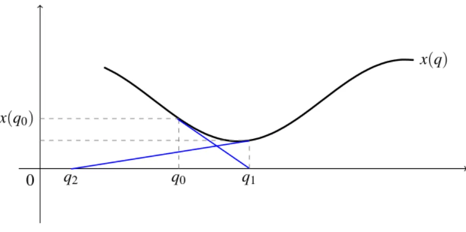
Gradient descent methods, such as Newton-Raphson algorithm, are subject to local extrema. Consider

for example the case represented in figure 2.4. The function x has a local minimum whose neighborhood

does not intersect the subspace x(q) = 0. At the minimum, the jacobian becomes singular, the product

JJ

gives an ill-conditioned matrix, which results in the divergence of the numerical method (see how

q

falls far from the local optimum).

0

x(q)

q

x(q

q

q

Figure 2.4: Divergence of Newton-Raphson algorithm near singularity

Near singularity, one method[Nakamura 1990] to avoid divergence is to perform a singular value decomposition on J and only invert the well conditioned part, discarding the singular directions. To do so, we decompose J as:

J

U





 σ₁

. ..

σ_m







V

then cancel the singular values below a chosen threshold and invert the ones above J

V

0

0 0

!

U

(2.9)

A second method[Nakamura and Hanafusa 1986] consists in replacing the optimization problem (2.5) by the following:







min

w

k

q

s.t J

q

x

w

(2.10) where k is a scalar. Minimizing the first part of the objective function tends to satisfy the linear constraint while minimizing the second part tends to keep a null update. Unless the linear constraint admits the null vector as solution, in which case it represents the optimum, the outcome of the optimization is a joint update with smaller norm than the one from (2.6). The importance of the second part of the objective function is scaled with k, directly influencing the norm of the optimal point, which is given by the formula:

δ

q

J

k

I

x (2.11)

The factor k

amplifies all eigen values of JJ

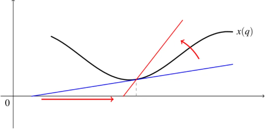
thus regulating the pseudo-inversion. To picture this process, consider a real function x and the tangent to its curve at point

x

q

x

x

When the derivative of x is not null, damping the inverse of x by a factor k

changes the tangent to:

(x^′)²+

k

x

q

x

x

We illustrate in figure 2.5 the effect of factor k

on the tangents near the singularity.

0

x(q)

Figure 2.5: Regulated pseudo-inversion: steeper tangents prevent large joint updates near singularity.

2.4 Prioritization

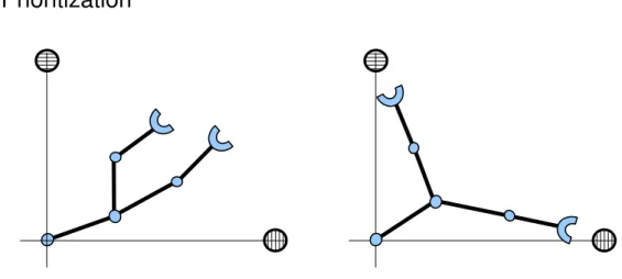
Figure 2.6: One target has to be prioritized to prevent failing both grasps.

Suppose that we seek the completion of two tasks x

0 and x

0 and that we cannot assess their feasibility without resorting to numerical resolution. Suppose, furthermore, that task 1 is more important that task 2. We derive the linear equations for differential kinematics:

J

q

x

(2.12)

J

q

x

(2.13)

Equation (2.12) has an affine subspace of solutions:

δ

q

s.t

q

J

x

J

J

z

(2.14) To express the absolute priority of task 1 with respect to task 2,

q is replaced in (2.13) giving the linear system:

δ

x

J

J

x

J

J

J

(2.15) Defining N

J

J

and

q

J

x

, the above linear system is solved in z:

(

min

z kδ

z

s.t

x

J

q

J

N

z

(2.16) yielding:

δ

q

J

x

N

N

J

q

which can be simplified to ([Nakamura 1990]):

δ

q

δq2

z }| {

J

x

| {z }

δq1

+(J₂

N

J

q

(2.17)

Figure 2.4 shows a representation of the successive orthogonal projections that lead to

q. To express the priorities, the second linear system is solved within the solutions of the first linear system, hence the second projection occurring inside the plane defined by the solutions of the first system. In case the tasks

J₁δq=δx₁

δq1

J₂δq=δx₂

δq₂ δq

Figure 2.7: Compatible tasks. The linear equality systems are compatible thus a solution satisfying both is found by successive pseudo-inversions.

are conflicting the union of linear systems is singular. The joint update

q satisfies the first linear system

and cannot satisfy the second. The regulated (2.11) or truncated (2.9) pseudo-inversion of the second

linear system ensures that the singularity does not yield a large update. The effect of both methods is

J₁δq=δx₁

δq1

J₂δq=δx₂

δq2

δq_reg

δq

(a) Regulation of the second pseudo-inversion gives a point between the solution to the first linear system and the solution to the normal pseudo-inversion of the second linear system.

J₁δq=δx₁

δq1

J₂δq=δx₂

δq2

δq

(b) Truncation of singular directions. The projection of the red line onto the plane represents the set of solutions to the truncated system.

Figure 2.8: Conflicting tasks. The red line represents the solutions of the linear system corresponding to the second task. The singularity of second task is represented by the near parallelism of the red line and the plane.

shown in figure 2.4.

The prioritization process is straightforwardly generalized to a set of k tasks. At priority level i, the solved optimization problem is:







min

w,δqi

k

w

k

q

s.t J

N

q

x

J

q

w

(2.18)

Based on this generalization, Algorithm 2 describes the steps taken to solve a set of prioritized linear equality systems. We propose the following compact formulation of the problem solved by this algorithm:

Find

q

solution to the optimization problem:











δ

min

q

s.t S

S

Arg min

δq∈S_i−1 k

J

q

x

(2.19)

Algorithm 2 calculates an update that acts on the values of all tasks simultaneously. Between two

consecutive stages ranked i and i+ 1, the joint update is modified to take into account the tasks at priority

level i without compromising the the tasks from level 1 to i

1. Like for the single task case, the linear

systems derived from the prioritized tasks are repeatedly solved by Algorithm 2 until convergence. The

convergence criterion takes into account all the tasks and observes their priority. It is shown in Algorithm

3.

Algorithm 2

Solve k prioritized linear equality systems

1:

n is the dimension of the kinematic structure

2:

N

I (n by n identity matrix)

3: δ

q

0 (n-sized null vector)

4: for

i

1 to k

5:

Calculate linear equality system (J

,

x

)

6:

J ˆ

J

N

7:

Calculate pseudo-inverse ˆ J

8: δ

q

J ˆ

x

J

q

9: δ

q

q

q

N

N

J ˆ

J ˆ

11: end for

2.5 Handling inequality constraints

Numerical inverse kinematics are used to control the motion of virtual characters, humanoid robots, etc. Most actuators on robotic systems only allow for a bounded range of motion between the connected bodies. Virtual characters also require joint limits to be observed for realism. Joint limits are naturally expressed as inequality constraints on the configuration:

in f

q

sup(q) (2.20)

and translate to joint update space as:

in f

q

q

sup(q)

q (2.21) which define an admissible convex volume in joint space outside of which a point corresponds to an update that would violate the joint limits. Naturally, the desired bounds for

q may be more constraining than in (2.21). From a geometrical point of view, pseudo-inversion is the computation of the orthogonal projection of a point onto an affine subspace. Nothing prevents the coordinates of the projection to fall outside the convex volume allowed by inequalities (2.21). Nonetheless, pseudo-inversion of a linear equality system is a fast operation that can be afforded for online robot control, animation of virtual figures in movies and video games. Therefore, modified versions of Algorithm 2 were proposed to account for joint limits.

One solution is to replace the optimization problem at every priority stage by the following one:







min

δ

q

W

q s.t J

q

x

(2.22)

Algorithm 3

Numerical inverse kinematics for k prioritized tasks

T

0, ...,T

0

1:

Define

the minimum task progression required to continue

2:

Call p the measure of task value progression

3: repeat

4:

5: for

i from 1 to k

6:

Calculate value of task i: T

7: end for

8:

9:

Solve the k prioritized linear systems [Algorithm 2]

10:

Update configuration q

q

q

11:

12: for

i from 1 to k

13:

Calculate value of task i: T

14:

Evaluate progression p

T

T

15: if

p

16:

break.

17: end if

18: end for

19:

20: until

p

W is a positive diagonal n-by-n matrix. The objective function here affects each degree of freedom in the configuration q with a weight w

. To emphasize this, the objective function can be written as:

n

∑

i=1

w

q

where

q

and w

are the i-th component of

q and w respectively. The larger the weight w

, the more

|δ

q

is minimized with respect to other coordinates, hence the idea: if

0 and q

is close enough to sup(q) then w

can be gradually increased to reduce the norm of

q

, making the corresponding joint brake before violating the upper limit. The same reasoning holds for the lower limit. The analytical solution to problem (2.22) is:

δ

q

J

x

=

W

J

J

x (2.23)

The weighted pseudo-inverse J

is what we would have obtained from the simple pseudo-inversion of the system:

J

W

q

x (2.24)

Expanding above equation into:

n

∑

i=1

√

1 w

∂

x

∂

q

q

x (2.25)

we could observe that the factor

wⁱ

scales the partial derivative of the task x, acting as brakes or

accelerator on the coordinate q

. The performance of this method relies essentially on the tuning of

the parameters w

with respect to the state of the kinematic structure.

The above method does not address the general case where any inequality constraint on

q might be considered. For example, bounding the velocity of a point P in the work space along vector d to remain below a maximal value c is written as:

d

P(q)

c from which an inequality constraint on the joint update follows:

d

J

q

c

where J

is the jacobian of the position of point P with respect to q.

There are solutions proposed by [Baerlocher 2001;

constraints within Algorithm 2. The inequality constraints are monitored after each priority stage and if violated, the stage is re-computed while taking the violated inequality constraints as hard equality constraints. This is the principle of active set algorithm. Supposing that priority stage i sees the system of inequality constraints A

q

b violated, the following optimization problem is solved instead of the usual problem (2.18):











w,

min

k

w

k

q

s.t J

N

q

x

J

q

w A

q

b

(2.26)

The resolution of 2.26 is repeated until the solution update of stage i,

q

, satisfies all the inequality constraints. The algorithm resumes its normal course afterward.

The main drawback of the method is the nested loop of pseudo-inversions that must be done at every stage to enforce the inequality constraints . There are more efficient algorithms to solve linearly constrained optimization problems with quadratic costs. As a matter of fact, other works[Zhao and

tasks into discrete priority levels was not available and the authors resorted to weighted sums of objective functions corresponding to several simultaneous tasks, such as:











min

w

J

q

x

s.t A

q

b

B

q

c

(2.27)

The weighted objective function does not permit strict enforcement of priority. When two of the

linear systems represented in the objective function cannot be solved simultaneously, the solution to

the minimization problem is a trade-off update that satisfies neither of the systems.

3

Generalizing priority to inequality tasks

3.1 Inequality task definition

Inequality tasks differ from inequality constraints in the way equality tasks differ from equality constraints. For a kinematic structure with n degrees of freedom, we have a differentiable kinematic property g : q

g(q) whose values are desired below a certain threshold, expressed without loss of generality in the following inequality:

g(q)

0 (3.1)

For a configuration q of the structure, if (3.1) is verified and is to be kept, it can be interpreted as a kinematic

call it a kinematic

One trivial example of inequality task can be g(q) = Hz(q)

0.5 where Hz(q) is the height of the robot hands from the ground. In this example, the task Hz(q)

0.5

0 requires the hands to be below the horizontal plane of equation z

0.5. Inequality tasks may be solved with Newton-Raphson algorithm like equality tasks through an iterative resolution of a linear differential system of inequalities. Defining J

q:

J

q

g(q)

(3.2)

19

The method of resolution of such systems is detailed in the next section. Continuing with the above example on the hand, equation (3.2) gives the following inequality:

∂

Hz

∂

q

q

0.5)

For a constant value of

and when the height of hands is below 0.5, the above equation sets a decreasing upper bound on the vertical hand velocity, a bound that is equal to 0 for z

0.5. Above the plane, the upper bound is negative and the plane z

0.5 acts as an attractor.

A linear inequality, when it has solutions, defines a halfspace. The set of solutions of a system of linear inequalities is the intersection of the half spaces generated by its inequalities. This set is a volume of

bounded by a convex polytope which may be closed or infinite (for example a half space is infinite). See figure 3.1 for an illustration of a system of linear inequalities in

.

I

I

I

x

x

Figure 3.1: The linear inequalities y

x and y

x determine the filled convex polytope.

One might observe that any equality task f

0 can be expressed as two simultaneous inequality

tasks, f

0 and f

0. Therefore inverse kinematics problems expressed as inequalities engulf

those that use equalities. One attractive aspect of inequalities is the possibility to specify a range or a

bounding on a kinematic property. What remains to be constructed is a framework that authorizes the

strict prioritization of inequality and equality tasks in any order. One may wonder about the scenarios

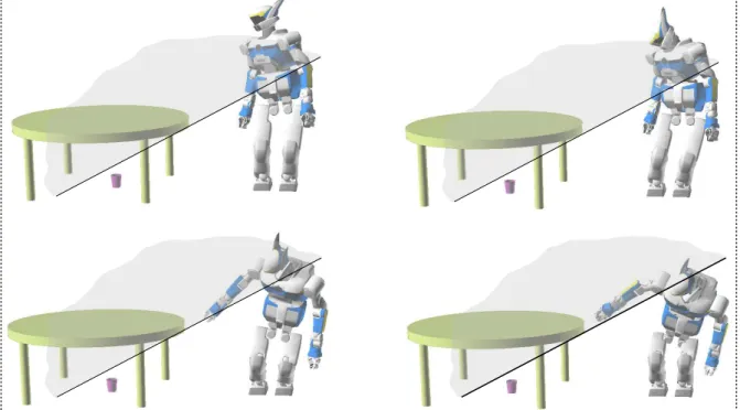
that require the inequality tasks to be at lower priority than equalities. Consider for example a humanoid

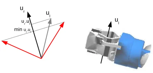
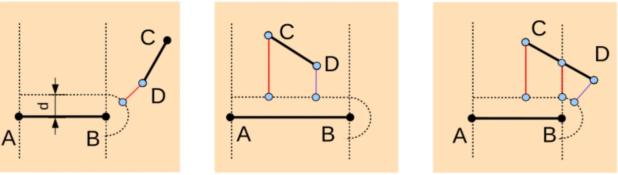
robot which has to grasp an object seen with embedded cameras. It is best if its reaching hand does not

come between the cameras and the object too soon. This is because we would like to keep checking the

visual target to maximize the chance of a successful grasp. In this scenario, the robot has to accomplish

a primary reaching task and a secondary region-avoidance task.

3.2 Description of the approach

Affecting priorities to linear systems means that we leave some of the systems unsolved to respect the ones with higher priorities. Letting L

and L

be two linear systems without common solutions, prioritizing L

over L

means that we retain a solution which satisfies L

to the expense of L

. Nonetheless, to take into account L

, one may select a solution of L

which minimizes the euclidean distance to L

’s solutions set. Euclidean distance is one example of optimality criterion adapted to systems of linear equalities. As a matter of fact, a point realizing this shortest distance belongs to the orthogonal projection of L

’s solutions on L

’s and can be obtained analytically. Furthermore, the entire set of points realizing the shortest distance may also be determined analytically [Nakamura 1990;

Siciliano and Slotine 1991]. To solve a third system of linear equalities

L

, the resolution is done within L

’s optimal set.

L

L

M P

Figure 3.2: The primary linear equality L

and a secondary system of 3 linear inequalities L

are without common solutions. M and P are solutions of L

minimizing the euclidean distance to L

’s set, however, P should be preferred since it satisfies two inequalities out of three while M satisfies none.

For our problem, we adopt the same approach consisting in solving every linear system in the optimal set defined by higher priorities. When we introduce systems of linear inequalities, however, we introduce solution sets which are volumes of

bounded by convex polytopes. In this particular case, euclidean distance is not a good optimality criterion (Figure 3.2). Therefore, we start by mapping equality and inequality tasks to suitable optimality criteria and study the nature of generated sets of solutions. We prove that the optimizations result in sets that can be described with linear systems and we deduce a resolution algorithm that is relatively easy to implement. This algorithm intended to prioritize inverse kinematics tasks can be straightforwardly applied to any problem involving the prioritization of a set of linear equality and inequality systems, regardless of the type of parameters. For this chapter, we will abandon the notations J and

q to emphasize the generality of the algorithm.

3.3 Mapping linear systems to optimization problems

In this section we construct optimization problems to solve each type of linear system. For each problem,

we demonstrate the nature of the optimal set.

Let A and C be matrices in

and b and d vectors in

with

. We will consider in the following either a system of linear equalities

Ax

b (3.3)

or a system of linear inequalities

Cx

d (3.4)

or both. When m

1, (3.3) is reduced to one linear equation and (3.4) to one linear inequality.

3.3.1 System of linear equalities

When trying to satisfy a system (3.3) of linear equalities while constrained to a non-empty convex set

, we will consider the set S

of optimal solutions to the following minimization problem:

min

1

2

w

(3.5)

with

w

Ax

b. (3.6)

Since the minimized function is coercive, the set S

is non-empty. We also have the property:

x

S

x

and Ax

Ax

(3.7) from which we can conclude that the set S

is convex.

Proof:

Let us consider an optimal solution x

to the minimization problem (3.5)-(3.6). The gradient of the minimized function at this point is

A

b).

The Karush-Kuhn-Tucker optimality conditions give us that the scalar product between this gradient and any vector v not pointing outside

from x

is non-negative,

w

Av

0 with

w

Ax

b.

Let us consider now two such optimal solutions, x

and x

. Since the set

is convex, the direction x

x

points towards its inside from x

, so we have

w

A(x

x

0 which is equivalent to

w

w

w

0.

The same can be written from x

,

w

w

w

0, so that we obtain

k

w

w

w

w

2w

w

0,

but this squared norm cannot be negative, so it must be zero and w

w

, what concludes the proof.

In the unconstrained case, when

, the solutions of (3.5)-(3.6) are such that A

Ax

A

b.

This minimization problem corresponds therefore to a constrained pseudo-inverse solution of the system of linear equalities (3.3).

3.3.2 System of linear inequalities

When trying to satisfy a system (3.4) of linear inequalities while constrained to a non-empty convex set

, we will consider the set S

of optimal solutions to the following minimization problem:

x∈Ω,w

min

1

2

w

(3.8)

with

w

Cx

d, (3.9)

where w plays now the role of a vector in

of slack variables. Once again, since the minimized function is coercive, the set S

is non-empty. Considering each inequality c

x

b

of the system (3.4) separately, we also have the property:

x

x

S

x

and

∀

j

(

c

x

d

c

x

d

c

x

d

c

x

c

x

(3.10) which means that all the optimal solutions satisfy a same set of inequalities and violate the others by a same amount, and from which we can conclude that the set S

is convex.

Proof:

Let us consider an optimal solution x

, w

to the minimization problem (3.8)-(3.9). The Karush-Kuhn-Tucker optimality conditions give that for every vector v not pointing outside

from x

,

w

Cv

0 and

w

max

0,Cx

d

(3.11)

This last condition indicates that if an inequality in the system (3.4) is satisfied, the corresponding element of w

is zero, and when an inequality is violated, the corresponding element of w

is equal to the value of the violation.

Let us consider now two such optimal solutions, x

, w

and x

, w

. Since the set

is convex, the

direction x

x

points towards its inside from x

, so we have w

C(x

x

0 which is equivalent to

w

d)

w

d)

0.

The optimality condition (3.11) gives

w

w

w

d)

and

w

w

w

d), so we obtain

w

w

w

0.

The same can be written from x

,

w

w

w

0, so that we obtain

k

w

w

w

w

2w

w

0,

but this squared norm cannot be negative, so it must be zero and w

w

, what concludes the proof.

3.3.3 Mixed system of linear equalities and inequalities

We can observe that systems of linear equalities and systems of linear inequalities are dealt with optimization problems (3.5)-(3.6) and (3.8)-(3.9) which have similar lay-outs and similar properties (3.7) and (3.10). The generalization of these results to mixed systems of linear equalities and inequalities is therefore trivial and we will consider in the following the minimization problem (in a more compact form)

min

x∈Ω,w∈ℜ^m

1

2

Ax

b

1

2

w

(3.12)

with

Cx

w

d. (3.13)

The set of solutions to this minimization problem shares both properties (3.7) and (3.10).

3.4 Prioritizing linear systems

3.4.1 Formulation

Let us consider now the problem of trying to satisfy a set of systems of linear equalities and inequalities

with a strict order of priority between these systems. At each level of priority k

1, . . . p

, both a

system of linear equalities (3.3) and a system of linear inequalities (3.4) are considered, with matrices

and vectors A

, b

, C

, d

indexed by their priority level k. At each level of priority, we try to satisfy these systems while strictly enforcing the solutions found for the levels of higher priority. We propose to do so by solving at each level of priority a minimization problem such as (3.12)-(3.13). With levels of priority decreasing with k, that gives:

S

(3.14)

S

Arg min

x∈Sk,w∈ℜ^m

1

2

A

x

b

1

2

w

(3.15)

with C

x

w

d

(3.16)

3.4.2 Properties

A first direct implication of properties (3.7) and (3.10) is that throughout the process (3.14)-(3.16), S

S

This means that the set of solutions found at a level of priority k is always strictly enforced at lower levels of priority, what is the main objective of all this prioritization scheme.

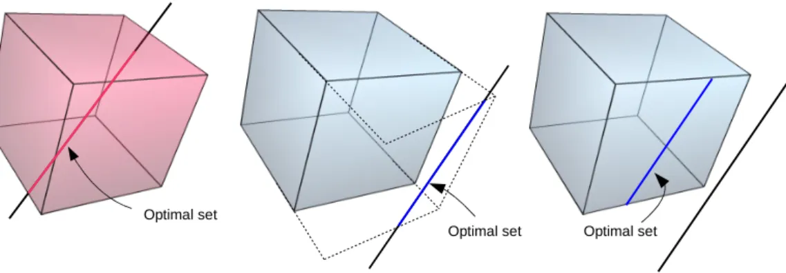
A second direct implication of these properties (3.7) and (3.10) is that if S

is a non-empty convex polytope, S

is also a non-empty convex polytope, the shape of which is given in properties (3.7) and (3.10). Figures 3.3 and 3.4.2 illustrate how these sets evolve in different cases. Classically, these convex polytopes can always be represented by systems of linear equalities and inequalities:

∀

k,

A ¯

b ¯

C ¯

d ¯

such that x

S

(

A ¯

x

b ¯

C ¯

x

d ¯

With this representation, the step (3.15)-(3.16) in the prioritization process appears to be a simple Quadratic Program with linear constraints that can be solved efficiently.

Note that when only systems of linear equalities are considered, with the additional final requirement of choosing x

with a minimal norm, the prioritization process (3.14)-(3.16) boils down to the classical problem 2.19.

3.4.3 Algorithms

The proposed Algorithm consists in processing the priority levels from highest to lowest and solving at every level the corresponding Quadratic Program. The representation of the sets S

by systems of linear equalities and inequalities is efficiently updated then by direct application of the properties (3.7) and (3.10).

It is naturally possible to optimize additional criteria over the final set of solutions. For instance, one

might be interested in the solution with minimal norm, or in the solution that maximizes the distance to

the boundaries of the optimal set, etc.

P1

P2

Optimal set

(a) Priority does not matter, the prioritized linear systems are compatible and the optimal sets is the intersections of their respective optimal sets.

P1

P2

Optimal set

(b) Equality has priority over inequality. The optimal set satisfies all possible inequalities while minimizing distance to the unfeasible ones.

P1

Optimal set