Contributions to Multi-Armed Bandits : Risk-Awareness and Sub-Sampling for Linear Contextual Bandits

(1)

HAL Id: tel-01277170

https://tel.archives-ouvertes.fr/tel-01277170

Submitted on 22 Feb 2016

HAL is a multi-disciplinary open access archive for the deposit and dissemination of scientific research documents, whether they are pub- lished or not. The documents may come from teaching and research institutions in France or

L’archive ouverte pluridisciplinaire HAL, est destinée au dépôt et à la diffusion de documents scientifiques de niveau recherche, publiés ou non, émanant des établissements d’enseignement et de recherche français ou étrangers, des laboratoires

and Sub-Sampling for Linear Contextual Bandits

Nicolas Galichet

To cite this version:

Nicolas Galichet. Contributions to Multi-Armed Bandits : Risk-Awareness and Sub-Sampling for Linear Contextual Bandits. Machine Learning [cs.LG]. Université Paris Sud - Paris XI, 2015. English.

�NNT : 2015PA112242�. �tel-01277170�

(2)

U NIVERSITÉ P ARIS -S UD

E COLE D OCTORALE D ’ INFORMATIQUE

L

ABORATOIRE DE

R

ECHERCHE EN

I

NFORMATIQUE

D ISCIPLINE : I NFORMATIQUE

T HÈSE DE DOCTORAT

Soutenue le 28 septembre 2015 par

Nicolas Galichet

Contributions to Multi-Armed Bandits:

Risk-Awareness and Sub-Sampling for Linear Contextual Bandits

Directrice de thèse : Michèle Sebag Directrice de recherche CNRS Co-directeur de thèse : Odalric-Ambrym Maillard Chargé de recherche INRIA Saclay Composition du jury :

Président du jury : Damien Ernst Professeur à l’Université de Liège (Belgique) Rapporteurs : François Laviolette Professeur titulaire à l’Université Laval (Québec)

Olivier Pietquin Professeur à l’Université Lille 1

Examinateurs : Damien Ernst Professeur à l’Université de Liège (Belgique)

Yannis Manoussakis Professeur à l’Université Paris-Sud

(3)

(4)

I State of the Art 17

3 Multi-armed bandits: Formal background 19 3.1 Position of the problem . . . 20

3.1.1 Notations . . . 21

3.2 The stochastic MAB framework. . . 22

3.2.1 Regrets . . . 23

3.2.2 Lower bounds . . . 24

3.3 The contextual bandit case . . . 25

3.3.1 Position of the problem . . . 25

3.3.2 Linear contextual bandit. . . 26

4 Multi-Armed Bandit Algorithms 27 4.1 Introduction . . . 28

4.2 Greedy algorithms . . . 28

(5)

4.2.1 Pure Greedy . . . 28

4.2.2 ε- greedy algorithm . . . 29

4.2.3 εt-greedy . . . 30

4.2.4 ε-first strategy . . . 30

4.3 Optimistic algorithms . . . 31

4.3.1 Upper Confidence Bound and variants . . . 32

4.3.2 Kullback-Leibler based algorithms . . . 34

4.4 Bayesian algorithms . . . 36

4.4.1 Algorithm description . . . 36

4.4.2 Discussion . . . 38

4.4.3 Historical study ofThompson sampling . . . 38

4.5 The subsampling strategy . . . 39

4.5.1 Introduction . . . 39

4.5.2 Definition . . . 39

4.5.3 Regret bound . . . 40

4.6 Contextual MAB Algorithms. . . 41

4.6.1 OFUL . . . 41

4.6.2 Thompson Sampling for contextual linear bandits . . . 42

4.6.3 LinUCB . . . 43

5 Risk-Aversion 45 5.1 Introduction . . . 45

5.1.1 Coherent risk measure . . . 46

5.2 Risk-Aversion for the multi-armed bandit. . . 47

5.2.1 Algorithms for the Mean-Variance . . . 47

5.2.2 Risk-Averse Upper Confidence Bound Algorithm . . . 51

II Contributions 55

6 Risk-Awareness for Multi-Armed Bandits 57 6.1 Motivations . . . 58

6.2 The max-min approach . . . 58

6.2.1 Algorithm definition . . . 59

6.2.2 Analysis . . . 59

6.3 Conditional Value At Risk: formal background . . . 64

6.3.1 Definitions . . . 64

6.3.2 Estimation of the Conditional Value at Risk. . . 66

6.4 The Multi-Armed Risk-Aware Bandit Algorithm . . . 67

6.4.1 Description . . . 67

6.4.2 Discussion . . . 67

(6)

III Conclusions 115

8 Conclusions and perspectives 117 8.1 Contributions . . . 117

8.1.1 Risk-Awareness for the stochastic Multi-Armed Bandits . . . 117

8.1.2 Sub-Sampling for Contextual Linear Bandits . . . 118

8.2 Future Work . . . 119

8.2.1 Improvements ofMARABOUTproof . . . 119

8.2.2 Risk-Aware Reinforcement Learning. . . 119

8.2.3 Extensions ofCL-BESA . . . 119

Appendices 121

(7)

A Résumé de la thèse 123

A.1 Introduction . . . 123

A.2 Regret . . . 124

A.2.1 Définitions . . . 125

A.2.2 Borne inférieure. . . 125

A.3 Prise en charge du risque . . . 126

A.3.1 Approche max-min . . . 126

A.3.2 Valeur à risque conditionnelle . . . 128

A.3.3 AlgorithmeMARABOUT . . . 131

A.4 Sous-échantillonage pour les bandit contextuels linéaires . . . 134

A.4.1 AlgorithmeCL-BESA . . . 134

A.4.2 Borne sur le regret contextuel . . . 136

A.4.3 Validation expérimentale . . . 137

A.4.4 Cadre expérimental. . . 138

A.4.5 Résultats . . . 138

A.5 Conclusion et perspectives . . . 139

(8)

List of Algorithms

1 Pure Greedy forK arms . . . 29

2 ε-greedy forK arms. . . 29

3 εt-greedy forK arms . . . 30

4 ε-first strategy forK arms . . . 31

5 UCBforK arms (Auer et al.,2002) . . . 32

6 UCB-VforK arms (Audibert et al.,2009) . . . 33

7 MOSSforK arms (Audibert and Bubeck,2010) . . . 34

8 kl-UCBforK arms (Cappé et al.,2013) . . . 36

9 Empirical KL-UCBforK arms (Cappé et al.,2013) . . . 37

10 Thompson samplingforK Bernoulli arms (Agrawal and Goyal,2012b) 37 11 Thompson samplingforK arms (Agrawal and Goyal,2012b) . . . 37

12 BESA(a,b) for two arms. . . 39

13 BESA(A) . . . 40

14 OFULfor K arms (Abbasi-Yadkori et al.,2011) . . . 41

15 Contextual linearThompson samplingforK arms . (Agrawal and Goyal, 2012a). . . 43

16 LinUCBforK arms. (Li et al.,2010) . . . 44

17 K-armedMVLCB . . . 49

18 K-armedExpExp . . . 51

19 RA-UCB(Maillard,2013) . . . 53

20 MINforK arms. . . 59

21 K-armedMARAB . . . 67

22 K-armedMARABOUT . . . 77

23 CL-BESA(a,b) for two arms . . . 91

24 CL-BESA(A) . . . 92

25 MARABpourK bras . . . 129

26 MARABOUTpourK bras . . . 132

27 CL-BESA(a,b) pour deux bras . . . 136

(9)

(10)

List of Figures

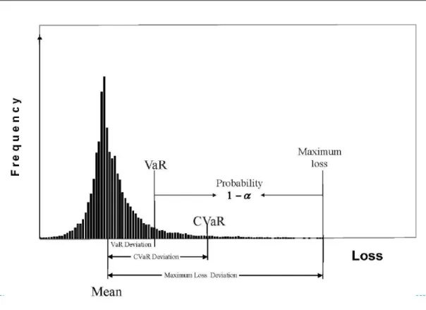
6.1 Illustration of an example of distribution satisfying the assumption of Equation 6.2.. . . 60 6.2 Value at risk and Conditional Value at Risk (fromRockafellar and Uryasev

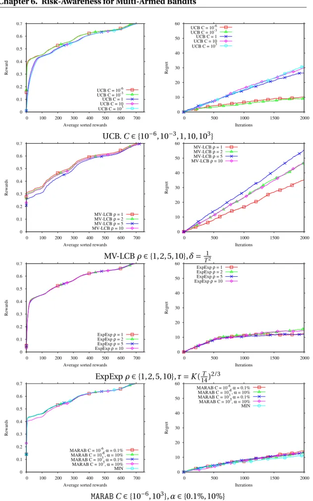
(2002)). . . 66 6.3 Cumulative pseudo-regret ofUCB,MINandMARABunder the assumptions

of Prop. 6.2.2, averaged out of 40 runs. ParameterC ranges in {10ⁱ,i=

−6 . . . 3}. Risk quantile levelαranges from .1% to 10%. Left: UCB regret increases logarithmically with the number of iterations for well-tunedC; MIN identifies the best arm after 50 iterations and its regret is constant thereafter. Right: zoom on the lower region of Left, withMINandMARAB regrets;MARABregret is close to that ofMIN, irrespective of theCandα values in the considered ranges. . . 70 6.4 Distribution of empirical cumulative regret ofUCB,MARAB,MVLCBand

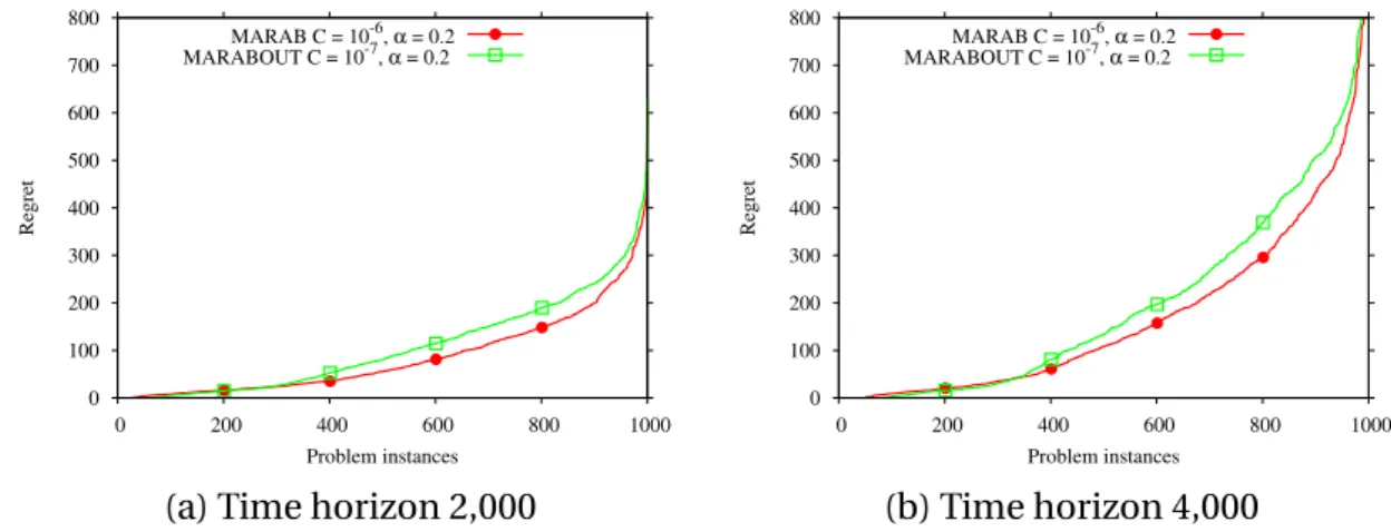
ExpExpon 1,000 problem instances (independently sorted for each algorithm) for time horizons T =2, 000 andT =4, 000. All algorithm parameters are optimally tuned (C=10⁻³forUCB,C =10⁻³forMARAB, α=20%,ρ=2,δ=_T¹2,τ=K(₁₄^T )^2/3). . . 72 6.5 Comparative risk avoidance for time horizonT =2, 000 for two artificial

problems with low (left column) and high (right column) variance of the optimal arm. Top:UCB; second row:MVLCB; third row:ExpExp; bottom:

MARAB. . . 74 6.6 Comparative performance ofUCB,MVLCB,ExpExpandMARABon a real-

world energy management problem. Left: sorted instant rewards (truncated to the 37.5% worst cases for readability). Right: empirical cumulative regret with time horizonT =100K, averaged out of 40 runs. . . 76 6.7 mCV aRPseudo-Regret forMARABOUTaveraged out of 100 runs, on three

2-armed artificial MAB problems (see text) withC∈©

10⁻⁴, 3ª

andβ=0.

Top row: problem 1 for time horizonT=200 (left) andT =2000 (right).

Bottom line: problem 2 (left) and problem 3 (right). . . 81

(11)

6.8 Comparative distribution of empirical cumulative regret ofMARABand MARABOUTon 1,000 problem instances (independently sorted for each algorithm) for time horizonsT=2, 000 andT =4, 000. . . 83 6.9 Comparative risk avoidance ofMARABandMARABOUTfor time horizon

T =2, 000 for two artificial problems with low (left column) and high (right column) variance of the optimal arm. . . 83 6.10 Comparative performance ofMARABandMARABOUTon a real-world en-

ergy management problem. Left: sorted instant rewards (truncated to the 37.5% worst cases for readability). Right: empirical cumulative regret with time horizonT=100K, averaged out of 40 runs.. . . 84 7.1 Contextual regret, in logarithmic scale as a function of the number of

iterations on the orthogonal problem with∆=10⁻¹,σX/p

2=∆,R_η=∆ ofCL-BESAfor various choices of the regularization parameterλ. Results averaged over 1000 runs. . . 106 7.2 Parameter influence on the contextual regret of OFULon the orthog-

onal problem with∆=0.1, (^σ^p^X

2,R_η)=(∆,∆) andλ=1. Left: R_{OFU L} ∈ {R_η, 10R_η, 100R_η},S_{OFU L}= ||θ||¯ 2. Right:S_{OFU L}∈{||θ||¯ 2, 10||θ||¯ 2, 100||θ||¯ 2}, R_{OFU L}=R_η. Results are averaged over 1000 runs. . . 108 7.3 Context perturbation and additive noise level:Contextual regret as a

function of the number of iterations on the orthogonal problem with

∆=10⁻¹ofCL-BESA,OFUL,LinUCBandThompson sampling.δOFU L= δT S=10⁻⁴,ROFU L=RT S=R_ηandSOFU L= kθk2(optimal values). Top to bottom:σX/p

2∈{₁₀^∆,∆, 10∆100∆}. Left:R_η=∆; Right:R_η=10∆. . . 112 7.4 Contextual regretofCL-BESA,OFUL,LinUCBandThompson sampling

as a function of the dimension on an orthogonal problem with ∆= 10⁻¹,σX/p

2=∆,R_η=∆,T =1000.δOFU L=δT S=10⁻⁴,R_{OFU L}=R_{T S}= R_ηandS_{OFU L,d}= kθdk2(optimal values). . . 113

(12)

Abstract

This thesis focuses on sequential decision making in unknown environment, and more particularly on the Multi-Armed Bandit (MAB) setting, defined by Lai and Rob- bins in the 50s (Robbins, 1952; Lai and Robbins, 1985). During the last decade, many theoretical and algorithmic studies have been aimed at the exploration vs exploitation tradeoff at the core of MABs, where Exploitation is biased toward the best options visited so far while Exploration is biased toward options rarely visited, to enforce the discovery of the true best choices. MAB applications range from medicine (the elicita- tion of the best prescriptions) to e-commerce (recommendations, advertisements) and optimal policies (e.g., in the energy domain).

The contributions presented in this dissertation tackle the exploration vs exploitation dilemma under two angles.

The first contribution is centered on risk avoidance. Exploration in unknown envi- ronments often has adverse effects: for instance exploratory trajectories of a robot can entail physical damages for the robot or its environment. We thus define the exploration vs exploitation vs safety (EES) tradeoff, and propose three new algorithms addressing the EES dilemma. Firstly and under strong assumptions, the MIN algorithm provides a robust behavior with guarantees of logarithmic regret, matching the state of the art with a high robustness w.r.t. hyper-parameter setting (as opposed to, e.g. UCB (Auer et al., 2002)). Secondly, the MARAB algorithm aims at optimizing the cumulative "Conditional Value at Risk" (CVaR) rewards, originated from the economics domain, with excellent empirical performances compared to (Sani et al., 2012a), though without any theoretical guarantees. Finally, the MARABOUT algorithm modifies the CVaR estimation and yields both theoretical guarantees and a good empirical behavior.

The second contribution concerns the contextual bandit setting, where additional informations are provided to support the decision making, such as the user details in the content recommendation domain, or the patient history in the medical domain.

The study focuses on how to make a choice between two arms with different numbers of samples. Traditionally, a confidence region is derived for each arm based on the associated samples, and the ’Optimism in front of the unknown’ principle implements the choice of the arm with maximal upper confidence bound. An alternative, pio-

(13)

neered by (Baransi et al., 2014), and called BESA, proceeds instead by subsampling without replacement the larger sample set.

In this framework, we designed a contextual bandit algorithm based on sub-sampling without replacement, relaxing the (unrealistic) assumption that all arm reward distributions rely on the same parameter. The CL-BESA algorithm yields both theoretical guarantees of logarithmic regret and good empirical behavior.

(14)

Remerciements

La thèse est une longue épreuve aussi enrichissante que difficile et que l’on ne peut aborder seul. Je réalise au moment de finaliser ce manuscrit la chance que j’ai eu d’être bien entouré et j’aimerais remercier toutes les personnes sans lesquelles cette thèse n’aurait pu être menée à bien.

• Merci aux membres de mon jury, qui m’ont fait l’honneur de se déplacer pour examiner mon travail. Merci à Damien ERNST et Yannis MANNOUSSAKIS.

Merci aux rapporteurs Olivier PIETQUIN et François LAVIOLETTE pour avoir pris le temps de réviser mon manuscrit.

• Merci à mes directeurs de thèse, Michèle et Odalric-Ambrym, pour leur disponi- bilité, leur patience, leurs conseils, leur aide et leur soutien indéfectibles.

• Merci à Olivier pour son aide précieuse à un moment clé de mon travail.

• Merci à Sophie LAPLANTE pour m’avoir orienté vers la recherche.

• Merci à tous les membres de l’équipe TAO d’hier et aujourd’hui pour les discus- sions (parfois scientifiques) et l’excellente ambiance. Merci à (par ordre alphabé- tique) : Adrien, Alexandre, Antoine, Asma, Aurélien, Basile, François, François- Michel, Gaétan, Jean-Baptiste, Jean-Joseph, Jean-Marc, Jérémie, Jérémy, Jialin, Karima, Lovro, Ludovic, Manuel, Marie-Liesse, Mouadh, Nacim, Olga, Riad, Sandra 1.0, Sandra 2.0, Sébastien, Simon, Sourava, Thomas, Vincent, Wassim, Weijia, Yoann. Merci à ceux que j’ai nécessairement oublié. Bonne chance et bon vent à ceux qui vont soutenir bientôt.

• Merci à FZ notre mascotte moustachue alsacienne et un clin d’oeil tout partic- ulier aux membres de son bureau, d’hier et aujourd’hui. Que son esprit perdure pour des générations de scientifiques.

• Merci et longue vie au PBA Crew !

• Merci à ma famille pour son soutien sans faille. Merci à mes parents, mes grands-parents, mes oncles, à mes soeurs Alice et Elsa, à mon frère Louis et à Marine.

(15)

(16)

Chapter 1 Introduction

Contents

1.1 Motivations . . . . 5

1.2 First problem statement . . . . 6

1.3 Applications . . . . 7

1.3.1 Clinical testing . . . 7

1.3.2 Algorithm selection. . . 7

1.3.3 Motor-Task Selection for Brain Computer Interfaces . . . 8

1.3.4 Web applications . . . 9

1.3.5 Monte-Carlo Tree Search . . . 10

1.4 Risk consideration in Multi-Armed Bandits . . . 12 Multi-armed bandits (MAB) (Robbins, 1952; Lai and Robbins, 1985) is a simple, generic however rich framework constituting the theoretical and algorithmic background of the work exposed in the present document.

1.1 Motivations

Originally, the termbandit(Thompson, 1933) refers to the casino slot machine as the MAB problem can be interpreted as an optimal playing strategy problem: a player enters a casino and is proposed a set of options orbandit armswith unknow associated payoffs. Given a fixed number of trials ortime horizon, his or her goal is to select arms in order to collect the highest amount of money possible.

While present under a wide variety of different settings, each of them emphazing specific learning aspects, the MAB framework is regarded as one of the most funda- mental formalizations of the sequential decision making problem, and in particular an illustration of theExploration vs. Exploitationdilemma:

(17)

• Exploration: The agent is assumed to have no prior information about the machine payoffs. This assumption implies the need for the agent to play, i.e. to explore, arms that were not or rarely tried.

• Exploitation: In order to gather the maximal amount of reward, the agent should play as often as possible, orexploit, the arms with estimated best payoffs.

In this respect, the MAB framework fundamentally differs from the statistical evaluation of the arm’s reward distribution. The goal is todiscriminatethe best options along the play, evaluation and interaction being donesimultaneously.

In particular, one focuses on the identification of the promising arms with the minimal number of samples, rather than on a precise estimation of every arm distributions.

The latter approach indeed provides useless information (tight estimates of suboptimal arms) at the cost of a high number of trials of these arms and lower cumulative rewards.

As said, the generic MAB framework allows many practical problems to be formalized and addressed using solutions from the bandit literature. Formally, any situation involving an agent repeatedly facing a choice between a given number of options with a priori unknown returns can be seen as a MAB problem. As this chapter aims to demonstrate, such situations occur frequently, explaining the rapidly growing body of literature in the MAB field. The scientific interest is also motivated by an accurate tradeoff between the expressivity and simplicity of the model allowing both a realistic and practically useful formalization and an in-depth theoretical study.

This chapter will present a few examples of MAB applications, starting with some definitions.

1.2 First problem statement

Standard notations are defined to introduce more formally some bandit applications.

The MAB setting considers a finite set ofK actions orbandit arms. Fori ∈{1 . . .K}, the i-th arm is associated with a reward distributionνi with expectationµidef

= E[νi]. At a given time stept, the agent choose, based on the previous observations, an arm I_t∈{1 . . .K} and observes an instantaneous rewardY_t∼νIt.

LettingT denote a finite time horizon (T ∈N^?), the agent’s goal is to maximize the cumulative sum of instantaneous rewards:

S=

T

X

t=1

Y_t (1.1)

(18)

1.3. Applications

1.3 Applications

This section presents some applications presented in the multi-armed bandit literature. This (far from exhaustive) list aims to illustrate the wide variety of successful applications of the MAB framework and motivate its study in the present document.

These example applications will also serve to illustrate our contributions, as discussed later on.

1.3.1 Clinical testing

Historically the introduction of the multi-armed bandit framework is due to Thomp- son, firstly considering a two-armed bandit problem (Thompson, 1933), then an arbitrary number of arms (Thompson, 1935). The studied problem considers a particular disease, with affected patients sequentially arriving. A (finite) set of drugs is available but their efficiency is unknown.

For each patient arriving (at timet), a drug is selected (I_t) and a reward (Y_t) is gathered depending on the efficiency of the treatment:Yt=1 if the treatment was effective, and 0 otherwise. In this clinical context, the relevance of the MAB setting is clear: as health and life are involved, it is vital to focus as quickly as possible on the best treatment rather than precisely determining the efficiency of every drug.

1.3.2 Algorithm selection

MAB has been used for Algorithm Selection in (Gagliolo and Schmidhuber, 2010).

Let us consider a binarydecisionproblem (e.g., SAT: for each problem instance, the decision problem is to determine whether this instance is satisfiable). Given a set B={b₁, . . . ,bM} of instances and a setA ={a₁, . . . ,aN} of algorithms/solvers¹, the goal is to iteratively pick an algorithm in order to minimize the time-to-solution.

By denotinglIt the time spent (loss) by the algorithmaIt on the instancebt presented at timet, a first formulation of this problem as a MAB problem is to consider the set of algorithms as the set of arms and to define the instantaneous reward asY_t = −l_I_t. This approach aims at the "single-best" algorithma^?∈A getting the best performance for everyinstanceb_m.

A refined setting considers a different set of arms, defined as Ktime allocators T A_j, mapping the history of collected performances of algorithms to a shares∈[0, 1]^N with P^N

i=1

s_i=1. The purpose of these time allocators is to run every algorithm inA in parallel on a single machine dividing the computational resource according to the

1The setAmay include a same algorithm/solver with different hyper-parameter settings.

(19)

shares. On a given amount of timeτ,s_iτis dedicated to algorithmi and the runtime associated with theT Aj is mini{^t_sⁱ

i}, withti runtime of algorithmi.

1.3.3 Motor-Task Selection for Brain Computer Interfaces

Brain-Computer Interfaces (BCI) are meant to provide a command law (e.g., of the computer or a wheeling chair) based the direct measurement of the brain activity.

These measurements rely on electroencephalography (EEG) or magnetoencephalogra- phy (MEG) technologies. One of the most promising applications of the BCI interfaces is to provide severely handicapped patients with controllable tools (e.g. robotic arm (Hochberg et al., 2012)).

Sensori-motor rhythms (SMR) are expressed and captured (via EEG) during the execution or imagination of a specific movement. SMRs thereby define a efficient way of communicating through BCI. (Fruitet et al., 2012) considers the training of such a SMR-based BCI to brain-control a single button when a given (imagined) movement is detected.

The problem can be decomposed into two steps. First a motor task has to be selected.

Based on this task, a classifier is learned in order to discriminate periods of (imagi- native) execution of the task and resting periods. One of the main challenges of this setting is the high variability of best movements depending on the studied patient.

The purpose of the approach thus is to discriminate the best taskwhileconstituting the classifier training sets.

The problem is defined by a numberK of tasks and a total number of rounds T. Note that these two quantities must be small in order to propose reasonable training sessions: long (largeN) or complex (largeK) sessions are to be avoided. In a bandit context, task are arms (in practice images to be displayed to ask the user to imagine a given task) andT is the time horizon. Instantaneous rewards areY_t are defined by the empirical classification rate associated to select taskIt∈{1, . . . ,K}.

The gain due to the MAB setting is explained by the early focus onusefuldiscrimina- tive tasks, through interaction with the user. Compared to the standard procedure ofuniformexploration, each task being presented an equal number of times, the approach proposed by (Fruitet et al., 2012) and based on the MABUCBalgorithm (presented in chapter4, (Auer et al., 2002)) showed benefits both in terms of classification rates (up to 18%) and training times (lowered by up to 50%).

(20)

1.3. Applications

1.3.4 Web applications

Document ranking

The MAB setting can be used to rank documents (Radlinski et al., 2008) and specifically web pages. The goal is to improve a web search engine performance by increasing the probability that users click on top-ranked results. This goal is formalized as follows. A fixed search query and a set of documentsD={d₁. . .d_n} is considered. At timet, an useru_t is proposed an ordered set of documentsB_t=(b₁(t), . . . ,b_k(t)) and clicks on documentd_i with probabilityp_t_i².

The goal is to avoid as much as possible theabandonmentphenomenon: no relevant document is presented and the request is unsatisfied.The instantaneous rewardY_t=1 if the user selects (clicks on) a documentd_i∈B_t andY_t=0 otherwise.

A first naive adaptation to the bandit framework would be to associate an arm to every possible orderedk−subset ofD, leading to MAB instance with _(n−k)!^n! number of arms.

The authors propose a more efficient method termedRanked Bandits Algorithm (RBA). The procedure relies on an preexisting MAB algorithm and runsk MAB instances (one per rank), each of these instances presentingnarms (one per document).

Thei-th MAB instance is in charge of choosing the document at ranki. In the case where thei-th MAB instance proposes an already selected document j for j <i, the choice is saved but another unpresented document is uniformly picked and presented.

After user clicks on documentb_i(t), MAB instances receive a 1 (resp. 0) reward ifb_i(t) was selected by the instance (resp. dismissed).

A key feature of this conception is its ability to produce diverse document rankings.

This property is desirable in such a context as methods assuming independent document relevances tend to output rankings with redundant documents, lowering the probability to present a relevant document to the user.

Content recommendation

MAB also is a natural framework for the recommendation and personalization of content (articles, advertisements, songs, videos . . . ) over Internet, which has been widely and intensively studed in the last decade (see for instance (Li et al., 2010;

Pandey and Olston, 2006; Babaioff et al., 2009; Agarwal et al., 2009; Kohli et al., 2013)), boosted by the need of many companies to assess the quality of a web-service and/or estimate the amount of advertising revenue.

The news article recommendation can be stated as follows. Visitors access a website and are proposed a selection of articles. The goal is to select relevant articles in order to maximize the probability to display at least an article of interest to the visitor. A

2Probabilitypt_iis conditioned by the user not clicking on documents ranked before documenti.

(21)

standard measure of performance in such problem is theClick-through rate(CTR) defined as the ratio ^{#cl i cks}#t r i al s.

A straightforward bandit adaptation would be to consider each possible pool of articles as a bandit armi and the rewardY_t=1 if an article is clicked at timetand 0 otherwise, leading to a setting close to the clinical testing one; this formalization could also be easily adapted to any other recommendation problem as it does not require any specific assumption regarding the content.

Nevertheless, a key feature of this setting is the important quantity of available information which can be used to efficiently improve the recommendations. Indeed, Web services often benefit from a vast amount of data (regarding the user’s interests or similar profiles) collected through over a long time and a large number of users.

This leads to the definition of theContextual banditframework, where side information is revealed to support the MAB decision process (Li et al., 2010). Contextual bandits will be further considered in Chapter 8, presenting the second contributions of this thesis.

Another MAB extension motivated by this application is proposed by Gentile et al.

(2014), who maintain user clusters in parallel of the recommendations. The underlying intuition is that similar users would have similar preferences, and information of similarity should be shared among users to improve recommendation.

1.3.5 Monte-Carlo Tree Search

The MAB setting has been used to guide exploration in a tree structure, enabling to extend their application to the selection of a (quasi-)optimal action in the broader context of a Markov Decision Process (MDP).

MDP is the main formalization used in Reinforcement Learning (RL, (Sutton and Barto, 1998; Szepesvári, 2010)), where an agent evolving in an unknown environment learns how to perform wellwhile interactingwith it. MDP is formalized by a tuple

¡S,A,P,R,γ¢

where:

1. S (resp.A) is thestate(resp.action) set.

2. P:S ×A×S →[0, 1] is the transition probability 3. R:S ×A×S →Ris the instantaneous reward function 4. γ∈[0, 1] is the discount factor

The goal is to find a (deterministic) policyπ:S →A, maximizing the cumulative reward overT (possiblyT = ∞)V^πdefined by

V^π(s)^def= E

"

T

X

t=0

γ^tR(s_t,a_t,a_t₊₁)|s₀=s,a_t=π(s_t)

#

(22)

1.3. Applications

Note that a MAB defines an MDP problem with a single state (thus without any dynamics), where the action setA is the (possibly large) set of arms.

The MAB setting was extended to the standard MDP setting, through a tree-structured exploration of the state space (Kocsis and Szepesvári, 2006b; Gelly et al., 2006). The approach makes the only assumption that a generative model of the MDP is available, allowing the sampling of states, actions and rewards; the best known algorithm to do so extends the Upper Confidence Bound (UCB, already mentioned (Auer et al., 2002)) to tree-structured search, defining theUpper Confidence bound applied to Trees (UCT) algorithm, where visited states are represented by tree nodes, and transitions by edges. Each node is associated with the cumulative rewards obtained by visiting the corresponding state.

Starting from the tree-root, UCT traverses the search tree in the following top-down way:

1. Considering the current state (tree node)s_i, the associated available actions and estimated rewards, the next actiona_iis selected thanks to a bandit algorithm (UCB).

2. Next states_i+1is determined from (s_i,a_i) using the generative model.

3. Ifs_i₊₁is a leaf, and the limit depth is not reached:

• a random actiona_i₊₁is selected and the arrivals_i₊₂state is provided by the generative model. The edge (a_i₊₁,s_i₊₂) is attached tos_i₊₁;

• a roll-out policy (e.g., uniformly random) selects next actions until a termi- nation condition is met (usually, when reaching a fixed horizonT);

• The cumulative rewardRassociated with the whole state-action sequence is computed;

• Information associated to visited nodes is updated thanks toR.

4. Otherwise, goto 1.

This procedure is repeated until reaching the prescribed numberN (budget) of time step; ultimately, it returns the action most visited at the top of the tree.

The MAB step achieves the iterative selection of actions (descendant nodes) at each stage of the search tree, leading to a search tree biased toward the most promising region of the search space. This feature offers a important double benefit, critical if the MDP problem involves large state and/or action spaces: it implies an efficient allocation of the computational resources and a reasonable memory usage.

(Kocsis and Szepesvári, 2006b) was the seminal work leading to the Monte-Carlo Tree Search(MCTS) family of algorithms. These algorithms received a considerable

(23)

scientific attention in the last decade due to their efficiency and genericity. Notable successes have been obtained in Computer Games, famous examples are Computer Go (Gelly et al., 2012) and Computer Hex (Hayward, 2009); in the latter game, artificial players now defeat human experts. The approach has also been applied to active learning (Rolet et al., 2009) or feature selection (Gaudel and Sebag, 2010) (among many others).

The interested reader is referred to (Browne et al., 2012) for an extensive survey of MCTS approaches and applications.

1.4 Risk consideration in Multi-Armed Bandits

As said, Multi-armed Bandits aim to discriminate and pull,as fast as possible, the arms with highest quality. This raises the central question of the relevant quality criterion.

Most authors in the MAB community consider the maximization of the expected payoff, where the goal is to identify and pull the arm with highestµi=E[νi] value. In some situations however, this criterion appears to be inappropriate. For instance in the clinical testing problem, let us one consider the following situation:

• A treatment A providing good results on average with rare lethal side effects.

• A treatment B providing slightly lesser results on average without any known side effect.

In such a situation, one would like to take into account another quality criterion, enforcing a more cautious exploration, at the expense of a potentially lower cumulative reward.

The general situation is even more critical as a large number of MAB algorithms are optimistic: they maintain a confidence region for the arm expected rewards and select the one with highest possible reward according to the information gathered so far. In the case of high variance on the distribution of the best arms, this would lead to a high number of pulls of arm with potentially low rewards.

In essence, in such a situation the usual tradeoff between exploration and exploitation must be extended to consider alsodecision safety. The exploration vs exploitation vs safety tradeoff will be further considered in Chapter 7, presenting the first contributions of this thesis.

(24)

Chapter 2

Overview of the contributions

The presented thesis proposes two main contributions to the Multi-Armed Bandits state of the art, summarized in this chapter.

2.1 Risk-Aware Multi-armed Bandit

ConsideringK arms with unknown reward distributionsνi, the mainstream MAB research is interested in maximizing the expected cumulative payoffs obtained after T trials. Equivalently, one is interested with minimizing thecumulative regret, sum of losses encountered comparatively to an oracle player. This problem has been extensively studied, both theoretically and empirically, leading to algorithms with proved optimal regret bound.

The limitation of the approach, in safety-critical situations, is to only consider the associatedexpectedpayoffµi of each arm. The associated theoretical guarantees require a sufficiently precise estimation of the arms’ payoffs, implying exploration efforts. In the case of high variances associated with the (best) arms, this leads to occasionally obtain extremely low payoffs. In many critical situations, these low payoffs must be avoided as they mean for instance the loss of expensive gears, the deterioration of patient’s health or even the loss of human lives.

The work presented in this manuscript propose mainly three contributions to the Risk-Aversion in the Multi-Armed Bandit setting, presented in Chapter6:

• Two criteria have been proposed for taking risk into account: the minimal value associated with each arm, and its Conditionnal Value at Risk (CVaR). The first one is the lower bound of the distribution support, the second is defined as the reward obtained in theα% worst cases,αbeing an user-defined parameter.

These criteria lead to designing three new algorithms:MIN,MARABandMARABOUT.

(25)

• The regret rates of MIN(Section6.2) andMARABOUT (Section6.6) have been theoretically studied.

• An extensive empirical study based on artificial MAB instances has been proposed, showing the benefits ofMINandMARAB(Section6.5)

• A real-world benchmark of energy allocation has been considered, confirming the gain obtained with risk aversion on moderate time horizons. (Section6.5.4).

2.2 Sub-Sampling for Contextual Linear Bandits

The second contribution presented in the manuscript concerns the contextual linear bandit setting.

Generalizing the stochastic MAB setting, Contextual Bandits considerK arms with unknown reward distributionsνi, where at each timet, a contextual informationX_t ∈ R^d is revealed to the learner and contributes to the computation of the instantaneous reward. The Contextual Linear model further assumes a linear dependency between X_t and the instantaneous rewardY_t. In the so-calleddisjoint model, one assumes the existence ofK vectorsθiassociated with each arm so that:

Y_t= 〈X_t,θIt〉 +ηt

withI_t the chosen arm at timetandηt an additive noise.

The contribution is to introduce the sub-sampling strategy first pioneered by (Baransi et al., 2014) in this setting. Sub-sampling bases the choice between two arms on equal quantities of information. Considering two arms denoteda andb with associated sampling sets (rewards and contexts) of respective sizesna andn_b, and assuming without loss of generality thatn_aÉn_b,n_asamples are uniformly drawn without replacement from the sampling set of armband the parametersθaandθbare estimated based each on a set of same sizen_a.

Although counterintuitive, this scheme has shown striking properties in the stochastic case, motivating its extension. In this regard, the contributions are

• The redefinition of an algorithm, termedCL-BESA, for the contextual case (Sec- tion7.2).

• The non-trivial derivation of a regret bound for a refined notion of regret (Section 7.3).

• An experimental validation on synthetic problem, illustrating the good empirical properties of the approach (Section7.4).

(26)

2.2. Sub-Sampling for Contextual Linear Bandits

The manuscript is organized as follows. The formal background and algorithms for the stochastic and contextual bandits are respectively presented in Chapters3 and4. Chapter5focuses on the notion of risk; it describes and discusses the state of the art concerned with risk-averse bandit algorithms. Chapter 6 presents our first contributions, and details algorithms based on the conditional value at risk, together with their theoretical and empirical analysis. Chapter7presents our second contributions, the extension of the sub-sampling technique to Contextual Linear Bandits. Finally, Chapter8concludes this manuscript by discussing the presented contributions, and describing future research directions.

(27)

(28)

Part I

State of the Art

(29)

(30)

Chapter 3

Multi-armed bandits: Formal background

Contents

3.1 Position of the problem . . . 20 3.1.1 Notations . . . 21 3.2 The stochastic MAB framework . . . 22 3.2.1 Regrets . . . 23 3.2.2 Lower bounds . . . 24 3.3 The contextual bandit case . . . 25 3.3.1 Position of the problem . . . 25 3.3.2 Linear contextual bandit. . . 26

This chapter introduces the formal background of the presented work, that is, the stochastic multi-armed bandit problem(MAB). After some definitions and notations, the different goals tackled by MAB settings are presented together with the associated evaluation criteria or loss functions known asregret. The chapter last presents the contextual MAB framework, which will be further considered in the manuscript. While there exists many other variants of the MAB setting, the chapter does not pretend to exhaustivity due to the fast growing literature devoted to the MAB settings and their extensions. The interested reader is referred to (Bubeck and Cesa-Bianchi, 2012) for a more comprehensive presentation of the related literature.

(31)

3.1 Position of the problem

Multi-armed Bandits (MAB), also referred to asK-armed bandit problem, consider an agent facingK independent actions, or bandit arms. Each arm is associated with an unknown, bounded, reward distribution. In each time step, the agent must select one of these arms on the basis of her current information about the arms and the associated distributions. Two main settings are studied:

• The best arm identification, where the agent is provided with a fixed budget (numberT of time steps) and must afterT trials decide for the arm that will be selected ever after. This setting is related to multipe hypothesis testing: the agent must decide for the best arm on the basis of the available evidence, and must select the evidence in order to do so with best confidence.

• The cumulative reward maximization, where in each time step the agent selects an arm and gathers the associated reward, with the goal of maximizing the sum of rewards gathered along time. In this second setting, the agent might know in advance the time budget (numberT of time steps, also calledtime horizon), or might consider the anytime setting where the agent performance is assessed as a function ofT, going to infinity.

This setting models the situation of a gambler facing a row of slot machines (also known as one-armed bandit), and deciding which arm he should pull in each time step, in order to maximize his cumulative gains.

It is seen that both settings define a sequential decision problem¹with finite or infinite time horizon, where the agent performance either is the sum of the rewards gathered in each time step (cumulative reward maximization), or the reward gathered in the final state (best arm identification). In particular, the Exploration vs Exploitation (EvE) trade-off is at the core of both MAB and RL settings:

• Exploitation: In order to maximize its performance, the agent should focus on the best options seen so far;

• Exploration: Still, focusing on the best options seen so far might miss some better options, possibly discarded due to unlucky trials².

1Accordingly, the MAB problem could be seen as a particular case of reinforcement learning (RL) problem (Sutton and Barto, 1998). A first difference is that MABs involve a single state whereas the RL decision takes into consideration the current state of the agent.

2A second difference between RL and MAB, and related to the fact that MABs involve a single state, is that the MAB agent must simply explore the other options while the RL agent mustplan to explore (Roy and Wen, 2014). Typically, the RL agent must revisit known states as these can lead to other states, which themselves need be explored. A comparative discussion between the specifics of the RL and MAB settings is however outside the scope of this manuscript.

(32)

3.1. Position of the problem

As mentioned in Chapter 1, both MAB settings are relevant to a vast number of applications, all related to optimal decision making under uncertainty and sequential design of experiments (Robbins, 1952), where the agent must make decisions with the antagonistic goals of optimizing its performance on the basis of the available evidence, and gathering more evidence.

3.1.1 Notations

Let us introduce the notations which will be used in the rest of the document.

K denotes the number of arms or options (K∈N^?);

νi denotes the (unknown) bounded reward distribution associated with thei-arm (fori=1 . . .K);

µi denotes the expectation ofνi(µi

def= IE[νi]);

µ^? is the maximum expectation taken over all arms (µ^?^def= max

i=1...Kµi);

i^? is an index (possibly not unique) such thatµi^?=µ^?(i^?in 1 . . .K);

∆i is the optimality gap of thei-th arm (∆i def

=µ^?−µi);

T denotes the time horizon (T∈N^?), which might be finite or infinite;

t denotes the current time step;

I_t is the arm selected at timet;

Y_t is the reward obtained at timet;

Xi,t is thet-th selected reward drawn from distributionνi;

N_i,t is the number of times thei-th arm has been selected up to timet (N_i_,t =

t

P

s=1

1I_I_t_=i).

Without loss of generality, it is assumed that each reward distributionνihas its support in [0, 1]; it belongs to the setM([0, 1]) of probability measures on [0, 1]. The main three MAB settings involve:

• Stochastic MAB, where all distributions νi are stationary and the reward Y_t gathered at time steptupon selecting armi =It is independently drawn from distributionνi.

(33)

• Adversarial MAB, where rewardY_t is decided prior to the agent’s decision by the adversary (Bubeck and Cesa-Bianchi, 2012). One distinguishes the case where the adversary is independent from the agent’s past actions (oblivious adversary), and the case where it depends on the past (non-oblivious adversary). The study of the adversarial setting provides worst-case guarantees about the pessimistic case where the environment plays against the agent (e.g. when considering financial engineering problems³);

• Markovian MAB, where arm distributionsνi evolve according to a on/off Markov process. In Gittins et al. (2011), the distribution only evolves when the arm is selected, and it is frozen otherwise; in restless bandits (Guha et al., 2010), the state of the underlying Markov process controlling the evolution of the arm distributions is only sparsely revealed to the agent. This setting, related to the Partially Observable Markov Decision Process setting, is relevant for applications in wireless scheduling and unmanned aerial vehicle (UAV) routing.

Only the stochastic and contextual MAB frameworks will be considered in the following of the manuscript.

3.2 The stochastic MAB framework

The stochastic MAB framework considers stationary reward distributions. At each time stept, the agent selects an armI_t∈{1 . . .K}; the environment draws rewardY_t according to distributionνIt, independently from the past, and reveals it to the agent.

As said, the MAB setting tackles one out of two goals:

• Maximizing the cumulative gain gathered along time, defined as:

X

t

Y_t

• Identify with a budget ofT trials, the best arm. In the best arm identification case, the agent selects armI_T based on the sampleY₁. . .Y_T₋₁(withY_t∼νi,i = I_t), thus with the goal of maximizingµIt.

The agent strategy (selecting an arm in each time step on the basis of the available evidence) is assessed in terms of regret compared to the optimal strategy. In the cumulative gain maximization (respectively in the best arm identification) problem, the optimal strategy, also called oracle strategy, selects in each time step (resp. at time

3Although empirical results suggest that the MAB strategies are too conservative, or equivalently, that the environment might be only moderately adversarial in such contexts.

(34)

3.2. The stochastic MAB framework

T) the best armi^?. It is clear that maximizing the agent performance is equivalent to minimizing its regret. One reason why the theoretical analysis considers the regret minimization (as opposed to, e.g., the cumulative gain maximization) in the literature is that the regret in some sense abstracts the difficulty of the problemper seand focuses on the quality of the strategy. For more difficult problems, even the oracle performance will be degraded; but the regret analysis only considers how much worse the strategy does, comparatively to the oracle.

3.2.1 Regrets

Three definitions of regret are introduced in the cumulative gain maximization case, respectively referred to as regret, pseudo-regret and empirical regret. In the last two cases, the rewards associated to the oracle strategy are simply set to their expectation, µ^?.

Definition 3.2.1(Cumulative regret). With same notations as above, thecumulative regretof the agent at time t is defined as:

R_t^def= max

i∈{1...K} t

X

s=1

X_i_,s−

t

X

s=1

Y_s (3.1)

and theexpected cumulative regret:

Eν1,...,νK[R_t]^def= E

·

i∈{1...Kmax} t

X

s=1

X_i,s−

t

X

s=1

Y_s

¸

(3.2) Definition 3.2.2 (Cumulative pseudo-regret). With same notations as above, the pseudo-cumulative regretof the agent at time t is defined as:

Rtdef

= Xt s=1

¡µ^?−µI_s

¢=tµ^?− Xt s=1

µI_s= XK i=1

∆iNi,t (3.3)

Definition 3.2.3(Empirical cumulative regret). With same notations as above, the empirical cumulative regretof the agent at time t is defined as:

cR_t ^def=

t

X

s=1

¡µ^?−Y_s¢

(3.4) Likewise, the regret defined for the best arm identification problem, called simple regret, measures the difference between the expectation of the true best arm, and the recommended arm:

Definition 3.2.4(Simple regret). Letting J_t denote the recommended arm after t trials,

(35)

thesimple regretr_t is defined as:

r_t^def= µ^?−µJt =∆Jt (3.5) The significant difference between both goals, the cumulative gain maximization and the best arm identification, concerns the related EvE tradeoffs, and the price of exploration as manifested in the different regrets (see Stoltz et al. (2011)):

• When considering the maximization of the cumulative gain, the exploration and the exploitation both take placeduring the T fixed trials; the role of exploration is to discriminate the non-optimal arms. The optimal regret rate, that is logarithmic in the budgetT after Lai and Robbins (1985), requires that non optimal arms are played at most a logarithmic number of times.

• On the other hand, the best arm identification involves two separated exploration and exploitation phases. The simple regret (eq. 3.5) minimization involves the pure exploitation of a single armafter a pure T-step exploration phase, and no loss is encountered during the exploration phase. It is said that thepureexploration phase is followed by a single exploitation phase, also called recommendation. (Stoltz et al., 2011) show that optimal rates are here conversely obtained for a linear number of suboptimal arm trials.

The regret is studied in the literature considering two main settings: the distribution- free (where no assumption is done about e.g. the moments of the underlying distributions) and the distribution-dependent settings. Typically, in the distribution-free setting, the loss incurred by selectingntimes thei-th arm cannot be higher thann∆i, whereas the (distribution-dependent) bounds on the regret depend on 1/∆i (since, the lower∆i the more easily one can mistake thei-th arm for the optimal arm).

3.2.2 Lower bounds

This section presents the main results on lower bound for the distribution-free and the distribution-dependent cases.

Theorem 1(Auer et al. (1995)). Letsupbe the supremum over all stochastic bandit bounded in[0, 1]andinfthe infimum over all forecasters, the following holds true:

inf sup E[R_t]Ê 1 20

pt K (3.6)

Definition 3.2.5(Kullback and Leibler (1951)). LetP([0, 1])be the set of probability distribution over[0, 1]. The Kullback-Leibler divergence between two distributions P

(36)

3.3. The contextual bandit case

and Q inP([0, 1])is defined as:

K L(P,Q)=





 R

[0,1]d P

dQlog_dQ^{d P}dQ if P ¿Q

+∞ otherwise (3.7)

A first version of the following theorem has been proposed by (Lai and Robbins, 1985) and then extended by (Burnetas and Katehakis, 1996).

Theorem 2(Burnetas and Katehakis (1996)). LetP ⊂M([0, 1)and a forecaster con- sistent withP,i.e. for any stochastic bandit, for any suboptimal arm i and anyβ>0, E[N_i,t]=o(T^β). For any stochastic bandit with distribution inP, the following holds true:

lim inf

T→∞

E[Rt] logt Ê X

i:∆i>0

∆i

K L(νa,ν) :ν∈P andE[ν]>µ^?ª

3.3 The contextual bandit case

3.3.1 Position of the problem

The contextual bandit differs from the canonical MAB setting as it is assumed that at each time step acontextis revealed to the agent. The agent strategy thus becomes to associate with each context an arm, in order to minimize the so-called contextual regret (below). The context, or side information, most naturally arises in some standard applications of MABs. For instance in the ads placement problem, the customer comes with some characteristic features (e.g., gender, age, location). One could see the contextual bandit as closer to the reinforcement learning setting, than the canonical MAB, by considering that thecontextcorresponds to some extent to the state of the agent. However the notion of dynamics in the state space, in relation with the action selection of the agent, is not present in the contextual bandit setting; still, the contextual bandit is a setting where the exploration / exploitation dilemma of the agent must take into account the current context.

In practice, contextual bandits are most often handled as a classification problem, associating with each context the arm yielding best reward for this context. Based on the information gathered during an exploration phase, one constructs a set of triplets (x_t,I_t,Y_t) which is used to learn how rewardY_tdepends on the contextx_tfor theI_t-th arm; this prediction is thereafter used to seek the arm yielding the maximum reward for a given context.

With same MAB notations as in Section3.1, let us introduce the notations related to Contextual Bandits. The contextual bandit adds side information in the form of a

(37)

contextvector from a given setX ⊂R^d. At each time stept∈N, a contextX_t∈X is drawn and revealed (e.g., in the case of a recommender system,Xt may be a vector summarizing the known information about the incoming user). Based on the information provided byX_t, the learner chooses an armI_t and observes an instantaneous rewardY_t (e.g., in the recommender system case, the arm set represents the different available contents, andY_tindicates whether the user clicks on the displayed contents).

3.3.2 Linear contextual bandit

In the linear contextual bandit case, one assumes that thei-th arm is associated with a (hidden) weight vectorθi, such that the instantaneous reward associated to thei-th arm is the scalar product of the context and the weight vector, augmented with some centered scalar noiseηt:

Y_t= 〈X_t,θIt〉 +ηt (3.9) with {θ1. . .θK} a set of unknown vector parameters inΘ⊂R^d.

The following additional assumptions are made:

• Firstly, it is assumed that contextsXt are independently drawn by Nature.

• Secondly, it is assumed that the parametersθi associated with each arm (to be estimated) are independent from each other. This scheme is calleddisjoint linear model(see (Li et al., 2010)); it differs from theOFUL(Abbasi-Yadkori et al., 2011) andThompson sampling(Agrawal and Goyal, 2012a) setting, where a common parameter is shared among the arms.

An algorithm based on sub-sampling for Linear Contextual bandit in the disjoint linear model will be proposed in Chapter7.

(38)

Chapter 4

Multi-Armed Bandit Algorithms

Contents

4.1 Introduction . . . 28 4.2 Greedy algorithms . . . 28 4.2.1 Pure Greedy . . . 28 4.2.2 ε- greedy algorithm . . . 29 4.2.3 εt-greedy . . . 30 4.2.4 ε-first strategy . . . 30 4.3 Optimistic algorithms . . . 31 4.3.1 Upper Confidence Bound and variants . . . 32 4.3.2 Kullback-Leibler based algorithms. . . 34 4.4 Bayesian algorithms . . . 36 4.4.1 Algorithm description . . . 36 4.4.2 Discussion . . . 38 4.4.3 Historical study ofThompson sampling . . . 38 4.5 The subsampling strategy . . . 39 4.5.1 Introduction . . . 39 4.5.2 Definition . . . 39 4.5.3 Regret bound . . . 40 4.6 Contextual MAB Algorithms. . . 41 4.6.1 OFUL . . . 41 4.6.2 Thompson Sampling for contextual linear bandits . . . 42 4.6.3 LinUCB. . . 43

(39)

4.1 Introduction

The many algorithms designed in the past decade to tackle the multi-armed bandit problem, specifically addressing the stochastic and the contextual MAB settings, can be divided into four categories:

1. Greedy algorithmsare mostly based on the exploitation of the best arm evalu- ated so far, with little to no exploration.

2. Optimistic algorithms: these algorithms rely on theoptimism in face of uncer- taintyprinciple. They use the reward samples to maintain a confidence region for every arm reward expectation, where the mean lies with a high probability.

The optimistic strategy consists of selecting the arm with highest possible mean reward based on the current knowledge.

3. Bayesian algorithms: These algorithms, mainly variants ofThompson sampling, maintain an estimated payoff distribution for each arm. Given a prior distribution on each arm, and the reward samples gathered every time the arm is selected, the posterior arm distribution is computed using Bayesian inference and the arm with maximal estimated expectation is selected.

4. Sub-Sampling based algorithm: Recently introduced in (Baransi et al., 2014), this algorithm selects the arm with best average reward, where the average estimate is based on an equal quantity of samples for each arm.

4.2 Greedy algorithms

This section is devoted to the presentation of some greedy MAB algorithms. After introducing a pure greedy method, some methods achieving an exploitation / exploration trade-off are presented and discussed. As will be seen in Chapters5and6, the simplicity of the greedy algorithms does not prevent them from being competitive in some settings.

4.2.1 Pure Greedy

The simplest strategy for the MAB problem consists of trying once each arm and greedily selecting the arm with best average reward ever after (Algorithm1).

The greedy, exploitation-only, approach is likely to miss the best arm. Consider for instance the 2-arm problem with Bernoulli distributionsν1=B(0.2) andν2=B(0.8).

It is clear thani^?=2. However, if unfortunately the first trials yieldY₁=1 andY₂=0, the pure greedy algorithm is bound to select the 1st arm ever after, yielding a linear