CoSenS reference guide Bilel Nefzi, Ye-Qiong Song

(1)

HAL Id: inria-00443594

https://hal.inria.fr/inria-00443594v2

Submitted on 16 Apr 2010

HAL

is a multi-disciplinary open access archive for the deposit and dissemination of sci- entific research documents, whether they are pub- lished or not. The documents may come from teaching and research institutions in France or abroad, or from public or private research centers.

L’archive ouverte pluridisciplinaire

HAL, est

destinée au dépôt et à la diffusion de documents scientifiques de niveau recherche, publiés ou non, émanant des établissements d’enseignement et de recherche français ou étrangers, des laboratoires publics ou privés.

CoSenS reference guide

Bilel Nefzi, Ye-Qiong Song

To cite this version:

Bilel Nefzi, Ye-Qiong Song. CoSenS reference guide. [Technical Report] 2009. �inria-00443594v2�

(2)

CoSenS reference guide

BILEL NEFZI AND YE-QIONG SONG

NANCY UNIVERSITY INPL, CAMPUS SCIENTIFIQUE - BP 239 – 54506 VANDOEUVRE-LES-NANCY CEDEX, FRANCE

{NEFZI, SONG}@LORIA.FR

INTRODUCTION

This report provides a reference guide to the CoSenS protocol stack. CoSenS provides a simple but efficient improvement of the MAC layer of IEEE 802.15.4 [1] in terms of reliability, delay and throughput. The network layer uses static routing or hierarchical tree routing of ZigBee standard [2].

The objective of CoSenS besides the improvement of IEEE 802.15.4 standard is to allow quality of service (QoS) support in wireless sensor networks. The MAC layer enables the implementation of scheduling policies and management mechanisms like congestion control and data aggregation.

PROTOCOL DESIGN

GENERAL PARAMETERS AND NETWORK ARCHITECTURE

We consider a wireless network composed of simple nodes and router nodes (named router in the rest of the document). A simple node is a device that generally has measurement sensors built in and has limited routing decisions capabilities. A router is a device that implements full routing and network management protocols.

However, it can act like a simple device when its routing and management capabilities are disabled.

The network may be statically defined or dynamically organized into a tree. In the latter case, it uses the tree addressing scheme presented in ZigBee standard.

CHANNEL ACCESS PROTOCOL

GENERAL DESCRIPTION

(3)

Fig. 1. An example of how the collecting and sending burst scheme operates

All nodes (simple nodes and routers) use CSMA/CA protocol to access the medium but with different maximum backoff intervals in order to give routers higher chance to access the medium; we used the unslotted version of CSMA/CA proposed by IEEE 802.15.4 (used in the non beacon enabled mode). CoSenS operates on the top of the "2450 MHz DSSS IEEE 805.15.4" physical layer; the data rate is equal to 250 kbps.

Routers use on the top of CSMA/CA protocol a collecting and sending burst scheme. In fact, a router does not transmit packets one by one upon their arrival. Instead, it waits for a period of time that we call waiting period (WP) and collects data either from its children or from its neighbor routers. After the end of the WP, the router starts transmitting all packets queued in its buffer in a single burst. We call this period of time the transmission period. Finally, at the end of the TP, the router starts another cycle and goes again to the waiting for reception state. WP and TP are illustrated in the example given by Fig. 1. Full details of the WP and TP are given next.

WAITING PERIOD

We define

 d_S and d_R as the maximum amount of time needed by a simple node and a router, respectively, to perform collision avoidance procedure (𝑑_𝐵𝑃), sense the channel (𝑡_CCA) and detect that it is Idle (at the first attempt), change the antenna state from receiver to sender (𝑡_tat ), send the packet (𝑑_pkt ), wait for an acknowledgment (𝑡_ack), and receive it. See Fig. 2.

 𝑁𝑚𝑎𝑥 as an integer which has a minimum value of 1. Its value depends on the amount of received traffic.

 𝑁_𝑐^𝑟 as the number of children associated to the router r.

Fig. 2. 𝐝𝐒, 𝐝𝐑 and ^𝟏

𝝁

𝑊𝑃 is given by the equation 2. When a router has no children, data packets come only from neighbor routers.

Hence, we use dR as a basis to calculate 𝑊𝑃 duration. In the other case, data packets can come either from children or neighbor routers. However, since d_S is greater than d_R (because 𝑑_𝐵𝑃 is bigger for simple nodes), it is used as a basis to calculate 𝑊𝑃 duration.

𝑊𝑃 = 𝑁𝑚𝑎𝑥 ∙ 𝑑S if 𝑁𝑐𝑟 ≠ 0 𝑁_𝑚𝑎𝑥 ∙ 𝑑_R 𝑜𝑡𝑕𝑒𝑟𝑤𝑖𝑠𝑒 (2)

(4)

ESTIMATION ALGORITHM

Let's define first the set Ω ∈ IN as the set of 𝑊𝑃s during which the router receives data and 𝑊𝑃_𝑘, 𝑘 ∈ Ω these 𝑊𝑃s. We define also, 𝑈_𝑘, 𝑘 ∈ Ω as the ratio giving the sum of the service times of received packets ( 𝑖∈𝐸_𝑘‍

1

𝜇_𝑖, 𝐸_𝑘 is the set of received packets during 𝑊𝑃_𝑘) divided by 𝑊𝑃_𝑘 duration. ¹

𝜇_𝑖 is the service time of packet 𝑖 (Fig. 2). 𝑈𝑘 is shown in (3). We note that 𝑈𝑘 can exceed 1 in the case where the router is still receiving a packet from a child or data from a neighbor router while the 𝑊𝑃 ends (recall that the router is not preemptive).

𝑈𝑘 =

𝑖 ∈ 𝐸𝑘‍1 𝜇 𝑖 𝑊𝑃_𝑘 (3) Let us denote by 𝑆𝑘 the exponential moving average of 𝑈𝑘, 𝑘 ∈ Ω

𝑆𝑘 = (1 − 𝛼)𝑆𝑘−1+ 𝛼𝑈𝑘 −1 (4)

𝛼 is the smoothing factor. We used a non linear filter where 𝛼 is bigger when 𝑈𝑘 −1 ≥ 𝑆𝑘 −1 allowing 𝑆𝑘 to adapt more swiftly to traffic increase. After a number of trials, we found that values of 𝛼, 𝛼1= 0.008 and 𝛼2= 0.01, gave the best of all-around performance. The computation of 𝑆𝑘 resembles that of the average queue length in RED [3] and the round trip time in TCP [4].

𝑆𝑘 is evaluated before the beginning of the 𝑘^𝑡𝑕 𝑊𝑃 and used in the Algorithm 1 to determine the value of 𝑁_𝑚𝑎𝑥 for the 𝑘^𝑡𝑕 𝑊𝑃 (thus its duration). In the algorithm, 𝑇𝑕𝑟_𝑚𝑎𝑥, 𝑇𝑕𝑟_𝑚𝑖𝑛 and 𝑁𝑀𝐴𝑋 designate the maximum threshold of 𝑆_𝑘, the minimum threshold of 𝑆_𝑘 and the maximum value of 𝑁_𝑚𝑎𝑥, respectively. 𝑇𝑕_𝑚𝑎𝑥 allows the increase of the WP's duration. When set too high, the WP will not respond rapidly to the network load growth.

When set too low, bandwidth will be wasted since the 𝑊𝑃 will increase too fast. 𝑇𝑕_𝑚𝑖𝑛 is the minimum utilization ratio under which the protocol performance will degrade significantly. 𝑇𝑕_𝑚𝑖𝑛 is used to decrease the WP's duration : set too high, WP decreases fast which diminish the benefits of our algorithm. When set too low, WP's duration decreases too slowly compared to the network load growth. The values of 𝑇𝑕𝑟_𝑚𝑎𝑥 and 𝑇𝑕𝑟_𝑚𝑖𝑛 are set to 0.28 and 0.75, respectively (tuned using some preliminary simulations with fixed WPs).

𝑁𝑀𝐴𝑋 bounds the value of 𝑁_𝑚𝑎𝑥 to prevent a high increase in the 𝑊𝑃 duration. It is set to 15 in all simulations.

/* Update 𝑆_𝑘*/

𝛼 = 𝛼1

𝒊𝒇 𝑈_𝑘−1≥ 𝑆_𝑘−1 𝒕𝒉𝒆𝒏 𝛼 = 𝛼₂

𝒆𝒏𝒅

𝑆_𝑘 = (1 − 𝛼)𝑆_𝑘−1+ 𝛼𝑈_{𝑘 −1}

/* Update 𝑁_𝑚𝑎𝑥*/

𝒊𝒇 (𝑆𝑘 ≥ 𝑇𝑕𝑟𝑚𝑎𝑥) 𝒕𝒉𝒆𝒏 𝑁_𝑚𝑎𝑥 = 𝑁_𝑚𝑎𝑥 + 1 𝒆𝒍𝒔𝒆

𝒊𝒇 (𝑆𝑘 ≤ 𝑇𝑕𝑟𝑚𝑖𝑛) 𝒕𝒉𝒆𝒏 𝑁_𝑚𝑎𝑥 = 𝑁_𝑚𝑎𝑥 − 1 𝒆𝒏𝒅

𝒆𝒏𝒅

𝑁_𝑚𝑎𝑥 = max(1, min(𝑁_𝑚𝑎𝑥, 𝑁𝑀𝐴𝑋))

Algorithm 1. Estimation algorithm

(5)

Intuitively, 𝑆𝑘 calculates the average utilization ratio of the 𝑊𝑃. If 𝑆𝑘 exceeds 𝑇𝑕𝑟𝑚𝑎𝑥, the value of the 𝑁𝑚𝑎𝑥 is increased which increases the duration of the 𝑊𝑃. If 𝑆𝑘 decreases below 𝑇𝑕𝑟𝑚𝑖𝑛, the value of 𝑁𝑚𝑎𝑥 is decreased. We can see that changing the 𝑊𝑃 duration, affects the value of 𝑈𝑘 (3) and so 𝑆𝑘 which in its turn affects the value of 𝑁_𝑚𝑎𝑥. Besides, 𝑆_𝑘 depends also on the traffic load. Hence, our algorithm appears like an iterative process where the objective is to find the good value of 𝑁_𝑚𝑎𝑥 that reflects the incoming traffic load while satisfying an utilization ratio between 𝑇𝑕𝑟_𝑚𝑖𝑛 and 𝑇𝑕𝑟_𝑚𝑎𝑥.

TRANSMISSION PERIOD

The collected data during the waiting period are transmitted in a burst. CSMA CA protocol is used to transmit only the first packet. Then, the remaining packets are transmitted directly upon the reception of the acknowledgement (𝑎𝑐𝑘)¹. If an 𝑎𝑐𝑘 is not received for a given packet, it is retransmitted using CSMA/CA protocol. Then, the remaining packets will be sent directly.

CoSenS needs a finite amount of time to process data received by the PHY. So, a separation period between the acknowledgment frame and the next transmission shall be used (however, they are fixed to zero in the simulations).

NETWORK LAYER

The network layer may use static routing or hierarchical tree routing (HTR) protocol defined in ZigBee standard.

In this section we describe the tree formation procedure and the HTR protocol.

NETWORK FORMATION

ASSOCIATION

We denote by the root, the router that starts the network and specifies all its parameters (like the parameters needed for address attribution). The root is equivalent to the the ZigBee coordinator in the ZigBee standard.

The association procedure works as follows. A node that wants to join the network, checks immediately its neighbor table to find the best candidate for association (the one that has the minimum depth and number of children). If a candidate is found, an association request is sent to this router. The node goes then to the waiting for reply state. If‍the‍neighbor‍table‍is‍empty,‍the‍node‍sends‍an‍“advertise_yourself” message, waits a defined amount of time and then checks the neighbor table again. The procedure is repeated until a candidate is found.

A router that receives an “advertise_yourself” message sends a hello message containing its address, depth, the number of its associated routers and the number of its associated simple nodes.

A router that receives an “association_request”‍ message and accepts the association, sends an

“association_response”‍ message to the originator of the request containing the assigned address and the network parameters.

The association messages are not acknowledged. A node that issued an “association_request” message waits a given amount of time for the “association_response” message. If it is not received, the whole procedure is repeated. During the association procedure, all application packets are destroyed.

1Acknowledgments are enabled in CoSenS

(6)

ADDRESS ATTRIBUTION

The network addresses are assigned using a distributed address allocation scheme that is designed to provide every potential parent with a finite sub-block of network addresses to distribute to its children. During network establishment, the root determines the maximum number of children per parent (𝐶𝑚), the maximum number of routers (𝑅𝑚) between these children as well as the maximum depth of the network (𝐿𝑚) (the root has a depth of 0). A function called 𝐶𝑠𝑘𝑖𝑝(𝑑) (equation 4) is used after that to calculate the size of the address sub- bloc being distributed by each parent located at depth 𝑑.

𝐶𝑠𝑘𝑖𝑝(𝑑) =

1 + 𝐶𝑚 ⋅ (𝐿𝑚 − 𝑑 − 1), 𝑖𝑓 𝑅𝑚 = 1

1+𝐶𝑚 −𝑅𝑚 −𝐶𝑚 ⋅𝑅𝑚^{𝐿𝑚 −𝑑−1}

1−𝑅𝑚 , 𝑜𝑡𝑕𝑒𝑟𝑤𝑖𝑠𝑒 (4)

The network address distribution is as follows. The root has always the address 0. For routers, the address assignment uses the value of 𝐶𝑠𝑘𝑖𝑝(𝑑) as an offset: if the node is the first served, its address is one greater than its parent address. Otherwise, the addresses are separated from each other by 𝐶𝑠𝑘𝑖𝑝(𝑑). For simple nodes, network addresses are assigned in a sequential manner using the following rule :

𝐴𝑛 = 𝐴𝑝𝑎𝑟𝑒𝑛𝑡 + 𝐶𝑠𝑘𝑖𝑝(𝑑) ⋅ 𝑅𝑚 + 𝑛 (5)

Here 1 ≤ 𝑛 ≤ (𝐶𝑚 − 𝑅𝑚) and 𝐴𝑝𝑎𝑟𝑒𝑛𝑡 represents the address of the parent.

HTR PROTOCOL

End devices (simple nodes in our case) always send their data to their father. For routers, HTR protocol is based on some comparison rules: for a ZigBee Router with address 𝐴 at depth 𝑑, if the following logical expression is true, then a destination device with address 𝐷 is a descendant.

𝐴 < 𝐷 < 𝐴 + 𝐶𝑠𝑘𝑖𝑝(𝑑 − 1) (6)

If it is the case, the Next Hop is given by the following rule:

 𝑁 = 𝐷 𝑓𝑜𝑟 𝑍𝑖𝑔𝐵𝑒𝑒 𝑒𝑛𝑑 𝑑𝑒𝑣𝑖𝑐𝑒𝑠 𝑤𝑕𝑒𝑟𝑒 𝐷 > 𝐴 + 𝑅𝑚 ⋅ 𝐶𝑠𝑘𝑖𝑝(𝑑)

 𝑁 = 𝐴 + 1 + ^{𝐷−(𝐴+1)}

𝐶𝑠𝑘𝑖𝑝 (𝑑) × 𝐶𝑠𝑘𝑖𝑝(𝑑) , 𝑜𝑡𝑕𝑒𝑟𝑤𝑖𝑠𝑒

If the expression is not true, the destination is not a descendant and the message should be routed through 𝐴's parent.

SIMULATION MODEL

NODE MODEL

CoSenS model is implemented within OPNET simulator [5]. The structure of the CoSenS sensor nodes (Fig. 3) used in the simulation model is composed of four functional blocks:

 The Physical Layer consists of a wireless radio transmitter (wireless_tx) and receiver (wireless_rx), operating at the 2.4 GHz frequency band and a data rate equal to 250 kbps. The transmission power is set to 0.05 W and the modulation technique is QPSK.

(7)

 The MAC Layer (mac) consists of an active queue where the server implements the CSMA/CA mechanism and the collect then send burst.

 The Network Layer (Nwk) implements the routing protocols and the association procedure.

 The Application Layer implements the traffic generator (gen) and the traffic sink (sink).

Fig. 3. Node model

Routers and simple nodes have the same node model but with different attributes. Table. 1 gives a summary of node attributes of routers and simple nodes.

Attribute Router Simple node

Acknowledgment Enabled Enabled

CSMA/C A

Minimum Backoff Exponent 2 3

Maximum Number of Backoffs 4 5

Collect then Send burst Scheme Enabled Disabled

Data generation Disabled Enabled

Table. 1. Node attributes

MAC MODEL

The MAC process model is illustrated in Fig. 4. It consists of two states, init and active. In the init state, all the model parameters are initialized. The active state handles all the received events. Every transition handles an event. The pair “(my_event)/my_function()” means that the event “my_event” is handled by the function

“my_function”. Here the list of the events.

 PHY_RECEPTION: Reception of a packet from the physical layer.

 TX_DONE: CSMA/CA process returns a transmission success.

 TX_FAILED: CSMA/CA process returns a transmission fail.

 SEND_TIMER: WP expired.

 ACK_TIMER: Acknowledgment timer expired

 NWK_RECPTION: Reception of a packet from the network layer

(8)

 Default: all other events

Fig. 4. MAC process model

CSMA/CA protocol is implemented as a process child of the MAC process. It is illustrated in Fig. 5. It is invoked either by bn_router_handle_nwk_msg() or bn_router_handle_tx_done() for simple nodes, bn_router_handle_send_timer_expiration() for routers and bn_router_handle_tx_failed() for both node types.

Fig. 5. CSMA/CA child process

NWK MODEL

The network process is illustrated in Fig. 6. It consists of three states; init, association and active. After the initialization phase (init) and depending on the routing protocol used, the model goes to the idle state or association state. The idle state handles all network events which are in our model, reception of an application layer packet (APL_RECEPTION) or an MAC packet (MAC_RECEPTION).

The association procedure is performed only when tree routing is used. The association model is implemented as a child process. It is illustrated in Fig. 7. It is invoked in the association state. The association protocol is described in the association subsection

(9)

Fig. 6. Network process model

Fig. 7. Association child process model

PERFORMANCE ANALYSIS

SIMULATION DESCRIPTION

In this set of scenarios, we will analyze the CoSenS performance regarding the self-synchronization between routers, end to end delay and throughput. The self-synchronization between routers is defined as the percentage of the simulated time where their TPs do not overlap.

For our simulations, the packet length is constant and equal to 400 bits. The generation is Poisson distributed.

Simulation duration is equal to 15min and all simple nodes start transmitting at t = 10 seconds (unless explicitly mentioned).

(10)

In the first seven sections we used static routing and varied the topology and number of destinations. The objective is to study the influence of these parameters on protocol performance. The eighth and ninth sections consider random networks with the use of HTR. The goal is to study the protocol performance under a more general topology. The last section analyzes the obtained results.

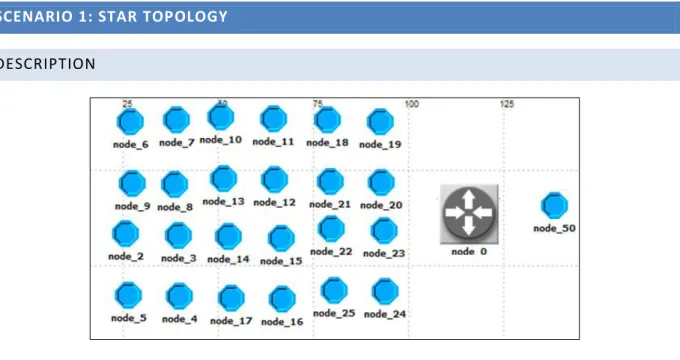
SCENARIO 1: STAR TOPOLOGY DESCRIPTION

Fig. 8. Star topology

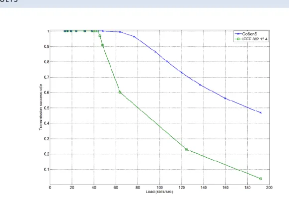
Nodes 6 to 24 send data to node 50 through the router 0. In this scenario we varied the inter arrival time and measured the transmission success rate and end to end delay.

RESULTS

Fig. 9. Successful transmission rate comparison between CoSenS and IEEE 802.15.4 for star topology.

(11)

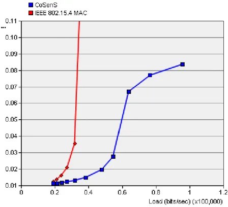
Fig. 10. End-to-end delay comparison between CoSenS and IEEE 802.15.4 for star topology.

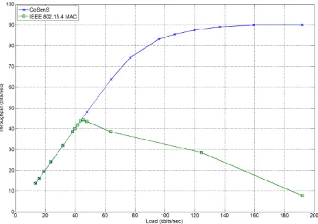
Fig. 11. Throughput comparison between CoSenS and IEEE 802.15.4 for star topology.

(12)

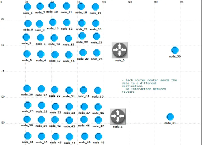
SCENARIO 2: TWO ROUTERS – SINGLE BROADCAST ZONE – TWO DESTINATIONS

DESCRIPTION

Nodes 6 to 24 are attached to router 0 and send data to node 50. Nodes 26 to 48 are attached to router 1 and send data to node 51. The inter arrival time is fixed to 0.3 seconds (~1.3 kb/s per node).

Fig. 12. Scenario 2.

RESULTS

SELF-SYNCHRONIZATION PERCENTAGE

Load (kb/s) 19.13 38.23 95.7

Self-synchronization 99.99 99.99 99.83

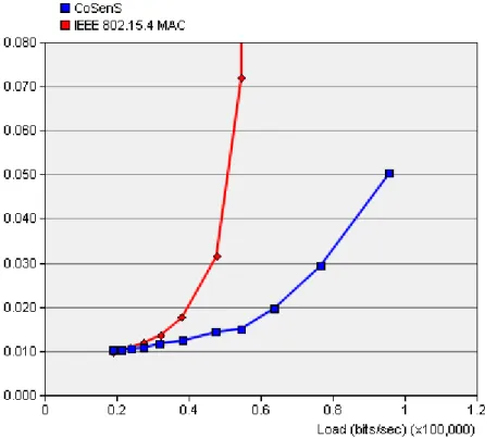
END TO END DELAY

(13)

Fig. 13. End to end delay (s) for scenario 2.

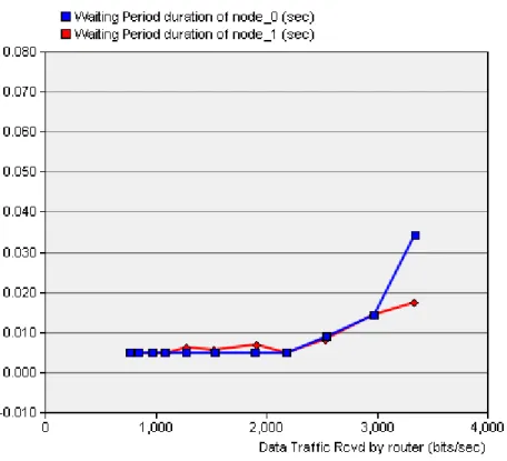
WP DURATION (IN SECONDS)

Fig. 14. Scenario 2 - WP duration.

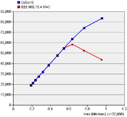
THROUGHPUT

(14)

Fig. 15. Throughput (bits/s) results for scenario 2.

(15)

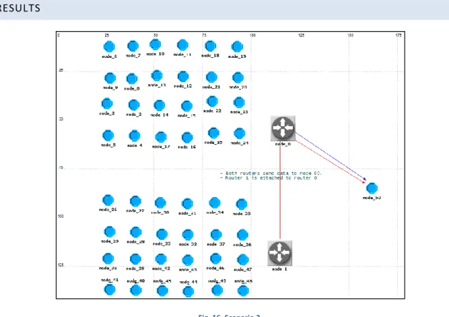
SCENARIO 3: TWO ROUTERS – SINGLE BROADCAST ZONE – ONE DESTINATION

DESCRIPTION

Two groups of nodes, each one attached to a router, send data to node_50 which is associated to node_0. So, node_1 forwards data to node_0. The inter arrival time is fixed to 0.3 seconds (~1.3 kb/s per node).

RESULTS

Load (kb/s) 18.93 38.22 95.73

Sef-synchronization 99.99 99.97 99.59

END-TO-END DELAY

The end-to-end delay increases in comparison with the first scenario since data generated by nodes 26 to 48 go through both routers to reach the destination.

(16)

Fig. 17. End-to-end delay (s) for scenario 3.

WP DURATION (FIG. 18)

Observe the increase of the WP duration for node_0 in comparison with scenario 2 as the data traffic received increases.

Fig. 18. WP duration for scenario 3.

(17)

THROUGHPUT (FIG. 19)

Fig. 19. Throughput (bits/sec) for scenario 3.

(18)

SCENARIO 4: FOUR ROUTERS – ONE BROADCAST ZONE – FOUR DESTINATIONS

DESCRIPTION

This scenario resemble scenario 2 but we added two node groups each one associated to one new router (Fig.

20). The inter arrival time is fixed to 0.5 seconds (~0.87 kb/s per node).

RESULTS

Load (kb/s) 19.25 54.25 95.86

Sef-synchronization (%) 99.98 99.96 98.27

END-TO-END DELAY

(19)

Fig. 21. End-to-end delay for scenario 4.

WP DURATION (FIG. 22)

It is the same for the four routers since they receive the same amount of data.

(20)

Fig. 23. Throughput for scenario 4.

(21)

SCENARIO 5: FOUR ROUTERS – ONE BROADCAST ZONE – TWO DESTINATIONS

DESCRIPTION

This scenario resemble scenario 3 but we added two node groups each one associated to one new router (Fig.

24).

RESULTS

Load (kb/s) 19.15 54.57 95.49

Sef-synchronization (%) 99.96 99.75 97.79

Fig. 24. scenario 5.

(22)

END-TO-END DELAY (FIG. 25)

WP DURATION (FIG. 26)

(23)

Fig. 27. Throughput for scenario 5.

(24)

SCENARIO 6: THREE ROUTERS – MULTIPLE BROADCAST ZONES – ONE DESTINATION

DESCRIPTION

This scenario is composed of three routers and four groups of children. Each two groups are associated to a router. The router in the middle does not have children and is used as gateway between the other ones. All nodes send data to a single destination (Fig. 28).

RESULTS

Load (kb/s) 19.15 54.57 95.49

Self-synchronization of node_0 and node_51 (%) 99.99 99.97 97.89 Self-synchronization of node_1 and node_51 (%) 99.99 99.95 97.53

(25)

END-TO-END DELAY

WP DURATION

(26)

THOUGHPUT (FIG. 31)

Fig. 31. Throughput (bits/sec) for scenario 6.

(27)

SCENARIO 7: MULTIPLE ROUTERS – MULTIPLE BROADCAST ZONES – MULTIPLE DESTINATIONS

DESCRIPTION

This scenario is composed of seven routers, six group of nodes (each one has 12 nodes) and four destinations organized as shown in Fig. 32.

RESULTS

END-TO-END DELAY

(28)

Fig. 33. End-to-end delay of scenario 7.

THROUGHPUT

Fig. 34. Throughput of scenario 7.

(29)

SCENARIO 8: RANDOM TOPOLOGY – MULTIPLE BROADCAST ZONES – ONE DESTINATION

DESCRIPTION

We consider the network illustrated in Fig. 35. It uses hierarchical tree routing (HTR). The root is 'node_0'. All nodes except node_0 are placed randomly. Two scenarios are simulated. In each one, all nodes send data to a different destination; the root for the first scenario and node_35 for the second one (delimited by circles in the figure).

TRANSMISSION SUCCESS PROBABILITY

Fig. 36. Transmission success probability of scenario 8.

(30)

END-TO-END DELAY

THROUGHPUT

(31)

SCENARIO 9: RANDOM TOPOLOGY2 – MULTIPLE BROADCAST ZONES – ONE DESTINATION

DESCRIPTION

We consider the network illustrated in Fig. 39. It is composed of 101 routers and 200 simple nodes uniformly distributed in a 1000m*1000m space. It uses the HTR routing protocol with the following parameters for network formation; Cm = 7, Rm = 4 and Lm = 7. The lines between routers represent the tree structure of routers (the tree structure of simple nods is not shown for figure clarity). The radio range is equal to 200m.

Simple nodes start transmitting at t=100s. This leaves enough time at the beginning of the simulation for network formation. We note that depending on the distance to the root node, nodes begin the association procedure at different times.

All simple nodes send data to the ROOT node located in the center of the network.

(32)

TRANSMISSION SUCCESS PROBABILITY

Fig. 40. Transmission success probability of scenario 9.

END-TO-END DELAY

(33)

THROUGHPUT

(34)

RESULTS ANALYSIS

All simulations scenarios show that the CoSenS provides better throughput, end to end delay and reliability than IEEE 802.15.4 MAC for medium and high traffic load. The results are similar for light traffic load. CoSenS ameliorates the weakness of CSMA/CA protocol namely the throughput, end to end delay and transmission success probability while preserving its simplicity and good scaling property. CoSenS is a collecting and sending burst scheme, the fact to queue the packets at routers allows us to design efficient scheduling algorithms, a key feature for providing differentiated QoS.

CONCLUSION

This report describes CoSenS in details and gives the results of some simulation scenarios which have been carried out to analyze its performance in comparison to IEEE 802.15.4 MAC using the unslotted CSMA/CA protocol. The results show that CoSenS greatly enhance throughput, end-to-end delay and reliability.

(35)

BIBLIOGRAPHY [5]

[1] IEEE TG15.4 (2006), Part 15.4: Wireless Medium Access Control (MAC) and Physical Layer (PHY) specifications for low-rate Wireless Personal Area Networks (LR-WPANs). IEEE standard for information technology..

[2] ZigBee Alliance, 473-489 ZigBee Specification Document 053474r17..

[3] S. Floyd and V. Jacobson, "Random Early Detection (RED) gateways for Congestion Avoidance ," in IEEE/ACM Transactions on Networking 1 (4), August 1993, p. 397–413.

[4] J. Postel, Transport Control Protocol, RFC 793. September 1981.

[5] OPNET Simulator, v14.5. http://www.opnet.com.