Développement d’un modèle météorologique multi-échelle pour améliorer la modélisation du climat urbain

HAL Id: tel-01002270

https://tel.archives-ouvertes.fr/tel-01002270

Submitted on 10 Jun 2014

HAL is a multi-disciplinary open access archive for the deposit and dissemination of sci- entific research documents, whether they are pub- lished or not. The documents may come from

L’archive ouverte pluridisciplinaire HAL, est destinée au dépôt et à la diffusion de documents scientifiques de niveau recherche, publiés ou non, émanant des établissements d’enseignement et de

multi-échelle pour améliorer la modélisation du climat urbain

Dasaraden Mauree

To cite this version:

Dasaraden Mauree. Développement d’un modèle météorologique multi-échelle pour améliorer la mod- élisation du climat urbain. Meteorology. Université de Strasbourg, 2014. English. �tel-01002270�

UNIVERSITÉ DE STRASBOURG

ÉCOLE DOCTORALE SCIENCES DE LA TERRE, DE L'UNIVERS ET DE L'ENVIRONNEMENT LABORATOIRE IMAGE VILLE ENVIRONNEMENT

THÈSE

présentée par :

Dasaraden MAUREE

soutenue le : 19 mars 2014

pour obtenir le grade de :

Docteur de l’Université de Strasbourg

: Sciences de la Terre et de l'Univers

Development of a multi-scale meteorological system to improve urban climate modeling

THÈSE dirigée par :

Prof. CLAPPIER Alain Professeur, Université de Strasbourg, France RAPPORTEURS :

Dr. HAUGLUSTAINE Didier Directeur de recherche, CNRS, France Dr. De RIDDER Koen Chercheur, VITO, Belgique

Dr. MARTILLI Alberto Chercheur, CIEMAT, Espagne

AUTRES MEMBRES DU JURY :

Dr. BLOND Nadège Chercheur, CNRS, France M. DESPRETZ Hubert Ingénieur, ADEME, France

R´esum´e

Ce travail a consist´e `a developper un mod`ele de canop´ee (CIM), qui pourrait servir d’interface entre des mod`eles m´eso-´echelles de calcul du climat urbain et des mod`eles micro-´echelles de besoin ´energ´etique du bˆatiment. Le d´eveloppement est pr´esent´e en conditions atmosph´eriques vari´ees, avec et sans obstacles, en s‘appuyant sur les th´eories pr´ec´edemment propos´ees. Il a ´et´e, par exemple, montr´e que, pour ˆetre en coh´erence avec la th´eorie de similitude de Monin-Obukhov, un terme correc- tif devait ˆetre rajout´e au terme de flottabilit´e de la T.K.E. CIM a aussi ´et´e coupl´e au mod`ele m´eso-´echelle WRF. Une m´ethodologie a ´et´e propos´ee pour profiter de leurs avantages respectifs (un plus r´esolu, l‘autre int´egrant des termes de trans- ports horizontaux) et pour assurer la coh´erence de leurs r´esultats. Ces derniers ont montr´e que ce syst`eme, en plus dˆetre plus pr´ecis que le mod`ele WRF `a la mˆeme r´esolution, permettait, par l’interm´ediaire de CIM, de fournir des profils plus r´esolus pr`es de la surface.

Abstract

This study consisted in the development of a canopy model (CIM), which could be use as an interface between meso-scale models used to simulate urban climate and micro-scale models used to evaluate building energy use. The development is based on previously proposed theories and is presented in different atmospheric conditions, with and without obstable. It has been shown, for example, that to be in coherence with the Monin-Obukhov Similarity Theory, that a correction term has to be added to the buoyancy term of the T.K.E. CIM has also been coupled with the meteorological meso-scale model WRF. A methodology was proposed to take advantage of both models (one being more resolved, the other one integrating horizontal transport terms) and to ensure a coherence of the results. Besides be- ing more precise than the WRF model at the same resolution, this system allows, through CIM, to provide high resolved vertical profiles near the surface.

Remerciements

Je tiens d’abord `a remercier Alain Clappier pour avoir dirig´e cette th`ese. Ses pr´ecieux conseils, ses explications et les innombrables tableaux remplis d’´equations ont ´et´e d’une grande utilit´e. Je le remercie aussi pour son amiti´e, sa compr´ehension, sa patience et “la petite cellule”.

Je tiens aussi `a remercier, tout particuli`erement, Nad`ege Blond, pour son en- cadrement, sa rigueur, son d´evouement sans faille et pour les discussions que nous avons eues durant ces derni`eres ann´ees. Je la remercie aussi pour ses conseils et les petits repas que nous avons faits.

J’adresse mes plus sinc`eres remerciements aux Dr. Didier Hauglustaine, Dr.

Koen de Ridder et Dr. Alberto Martilli pour avoir accept´e de juger et de donner leur avis sur ce travail. Je remercie aussi le Dr. Alberto Martilli pour les discussions que nous avons eues.

Merci `a M. Hubert Despretz, ing´enieur ADEME, qui a suivi cette th`ese, pour ses conseils et pour sa confiance. Je remercie aussi Mme. Val´erie Pineau de la cellule th`ese de l’ADEME. Merci aussi `a Mme. Aur´elie Gr´egoire de la R´egion Alsace pour le suivi de cette th`ese.

Je remercie aussi la direction du Laboratoire Image Ville Environnement de m’avoir permis d’effectuer ma th`ese.

Un merci tout particulier `a Estelle Baehrel pour sa pr´esence, son ´ecoute at- tentive et qui a toujours une solution `a nos probl`emes adminstratifs. Merci aussi

`a tous ceux qui ont contribu´e de pr`es ou de loin `a l’aboutissement de ce travail au laboratoire et `a la Facult´e de G´eographie. Merci aux personnes qui ont con- tribu´e au support technique de cette th`ese en particulier Romaric David et Michel Ringenbach. Je remercie, par ailleurs, Tajaneh et Ali, pour leur gentillesse.

Merci aux Jardins des Sciences de l’Universit´e de Strasbourg, tout partic- uli`erement Said, Christelle et Natasha, pour m’avoir permis de d´ecouvrir une autre fa¸cade de la recherche.

Je remercie aussi mes anciens coll`egues de bureau, Manon et Sajjad et mes nouveaux coll`egues Jana et J´er´emy pour m’avoir encourag´e pendant ces quelques mois et pour nos discussions sans fin. Merci `a Richard pour son soutien au cours des derniers mois et pour les petites escapades dans une autre r´ealit´e. Merci aussi

midi souvent folkloriques.

Je tiens `a remercier ma famille et mes amis, en France, en Suisse, en Angleterre, en Allemagne, aux Etats Unis et `a Maurice pour leur soutien au cours de ces derni`eres ann´ees. Un merci tout particulier `a mes parents, `a mon fr`ere et `a ma soeur qui ont toujours ´et´e pr´esent `a mes cot´es. Merci `a Kreena, Kurveena et Sevahnee pour leurs supports et leurs amiti´es.

Pour finir, merci `a Jevita pour son soutien. Nous avons v´ecu la mˆeme chose aux mˆemes moments. Comme tu le dis si bien: `a deux c’est beaucoup mieux et plus facile!

Cette th`ese a ´et´e financ´e par l’Agence de l’Environnement et de la Maˆıtrise de l’Energie, la R´egion Alsace et la Zone Atelier Urbaine Environnementale et a b´en´efici´e du soutien financier du R´eseau Alsace de Laboratoires en Ing´enierie et Sciences pour l‘Environnement (REALISE) pour l’achat de mat´eriel informatique.

Contents

1 Introduction 1-1

1.1 Climate change and building energy consumption . . . 1-1 1.1.1 Global Climate Change. . . 1-1 1.1.2 Urban development . . . 1-2 1.1.3 Adaptation and mitigation strategies . . . 1-3 1.2 Objectives . . . 1-4 1.3 Structure of the thesis . . . 1-5

2 On the need for a canopy model 2-1

2.1 Introduction . . . 2-1 2.2 From the Global to the Building scale . . . 2-2 2.2.1 Global . . . 2-3 2.2.2 Meso-scale . . . 2-4 2.2.3 Neighborhood and Street scale . . . 2-9 2.2.4 Building scale . . . 2-10 2.3 Interactions and feedbacks . . . 2-11 2.4 Models . . . 2-12 2.4.1 Meso-scale models . . . 2-13 2.4.2 Micro-scale models . . . 2-18 2.5 Limits of existing models . . . 2-20 2.6 Conclusion . . . 2-22 3 Development of a 1D-CANOPY model. Part I: Neutral case and

comparison with a C.F.D 3-1

3.1 Introduction . . . 3-1 3

3.3 Canopy Interface Model . . . 3-6 3.3.1 Governing Equation: Momentum Equation . . . 3-7 3.3.2 1.5 order turbulence closure . . . 3-8 3.3.3 Coherence between formulations of the turbulent diffusion

coefficient . . . 3-9 3.3.4 Governing Equation: Turbulent Kinetic Energy Equation . . 3-9 3.3.5 Discretization . . . 3-12 3.3.6 Obstacles integration . . . 3-13 3.4 Experiments with CIM . . . 3-17

3.4.1 Comparison of CIM with an analytical solution over a plane surface . . . 3-17 3.4.2 Scenarios to evaluate the impact of obstacles . . . 3-17 3.4.3 Comparison of CIM with a C.F.D model over an array of

buildings . . . 3-18 3.5 Results in neutral atmospheric conditions . . . 3-19 3.5.1 Without obstacles. . . 3-20 3.5.2 With obstacles . . . 3-20 3.6 Discussions and Conclusion . . . 3-25 4 Development of a 1D-CANOPY model. Part II: Stable and Un-

stable case - modification brought to the T.K.E equation 4-1 4.1 Introduction . . . 4-1 4.2 Monin-Obukhov Similarity Theory . . . 4-2 4.3 CIM developments considering atmospheric stability . . . 4-4 4.3.1 Turbulent diffusion coefficient and condition of a coherence . 4-5 4.3.2 Momentum . . . 4-6 4.3.3 Energy . . . 4-6 4.3.4 Turbulent Kinetic Energy . . . 4-7 4.3.5 Coherence over a plane surface . . . 4-9 4.3.6 Atmospheric stability . . . 4-12 4.4 Experiments with CIM . . . 4-12 4.5 Comparison of CIM with the MOST over a plane surface . . . 4-13

4.5.1 Results from the MOST . . . 4-13 4.5.2 CIM with a traditional formulation of the T.K.E. . . 4-14 4.5.3 CIM using the CG correction of the T.K.E equation . . . 4-14 4.6 Results with obstacles . . . 4-17 4.7 Discussions and Conclusion . . . 4-22 5 Multi-scale modeling of the urban meteorology: integration of a

new canopy model in WRF model 5-1

5.1 Introduction . . . 5-1 5.2 Weather Research and Forecasting model . . . 5-4 5.2.1 Governing equations and turbulent closure . . . 5-5 5.2.2 Focus on specific physics schemes . . . 5-6 5.3 Canopy Interface Model integration in WRF . . . 5-7 5.3.1 Canopy Interface Model . . . 5-8 5.3.2 WRF-CIM coupling strategy . . . 5-8 5.4 Experiments with WRF-CIM . . . 5-12 5.5 Results . . . 5-13 5.5.1 Global comparisons on specific vertical levels . . . 5-13 5.5.2 Comparison on specific vertical profiles . . . 5-17 5.5.3 Computational time . . . 5-24 5.6 Discussions and Conclusion . . . 5-24

6 Conclusions and Perspectives 6-1

6.1 Conclusions . . . 6-1 6.2 Perspectives . . . 6-3

7 R´esum´e en fran¸cais 7-1

7.1 Le changement climatique et les d´epenses ´energ´etiques des bˆatiments 7-1 7.1.1 Changements climatiques globaux . . . 7-1 7.1.2 D´eveloppement urbain . . . 7-2 7.1.3 Strat´egies d’adaption et d’att´enuation. . . 7-3 7.2 Mod`eles existants . . . 7-4 7.3 Objectif de la th`ese . . . 7-5

comparaison avec un mod`ele C.F.D . . . 7-6 7.5 D´eveloppement d’un mod`ele de canop´ee. Partie 2: cas stable et

instable, modification de la l’´energie cin´etique turbulente . . . 7-8 7.6 Mod´elisation multi-´echelle de la m´et´eorologie urbaine: int´egration

de CIM dans le mod`ele m´et´eorologique WRF . . . 7-9 7.7 Conclusions et perspectives. . . 7-16

List of Figures

1.1 Carbon dioxide concentration at Mauna Loa Observatory from 1960 to 2011. . . 1-1 1.2 World urban and rural population (in billions) from 1950 to 2050

[UN, 2012] . . . 1-2 1.3 Energy consumption in urban areas by sectors [ADEME, 2012] . . . 1-3 2.1 Structure of the Atmosphere (taken from www.ncsu.edu) . . . 2-1 2.2 Planetary Boundary Layer . . . 2-1 2.3 Evolution of the boundary layer during a diurnal cycle . . . 2-4 2.4 Example of an idealized Urban Heat Island - Temperature profile

above an urban area (taken from http://www.uta.edu) . . . 2-6 2.5 Multi-scale climate interactions (Global scale to micro-scale) . . . . 2-11 2.6 Interactions between the meso-scale and building (micro-scale) (Voogt,

2007) . . . 2-12 2.7 Representation of the urban canopy: left: single layer and right:

multi-layer . . . 2-16 2.8 Grid in a meso-scale model . . . 2-18 2.9 Grid in a micro-scale model . . . 2-19 3.1 Use of a canopy module allows low vertical resolution (results from

Muller, C., 2007) Bold black line (-) high resolution (20m) in meso- scale model; dotted line (- -) canopy model in meso-scale with low resolution (60m); pale black line (-) meso-scale model with low res- olution (60m) . . . 3-2

7

length andWx andWy are the street width in thexandy-directions respectively. dx and dy are the horizontal grid resolution while dz is the vertical resolution) . . . 3-13 3.3 Side view of a section of the 1-D column showing the interpretation

of porosity by CIM . . . 3-13 3.4 Comparison of the wind (in ms⁻¹) and T.K.E (in m²s⁻²) profiles

computed using the analytical solution from the Prandtl surface layer theory and CIM. Altitude is in meter. . . 3-20 3.5 Comparison of the wind (in ms⁻¹) and T.K.E (in m²s⁻²) profiles

computed to evaluate the impact of the obstacle porosities (with 25% and 75% of empty space in a grid cell). Altitude is in meter. . 3-21 3.6 Comparison of the wind (in ms⁻¹) and T.K.E (in m²s⁻²) profiles

computed to evaluate the impact of obstacles roof surfaces. Altitude is in meter. . . 3-22 3.7 Comparison of the wind (in ms⁻¹) and T.K.E (in m²s⁻²) profiles

computed to evaluate the impact of obstacles vertical surfaces. Al- titude is in meter. . . 3-23 3.8 Comparison of the wind (in ms⁻¹) and T.K.E (in m²s⁻²) profiles

obtained with obstacles from CIM and the C.F.D experiment with the mixing length equal to the height. Altitude is in meter. . . 3-24 3.9 Comparison of the wind (in ms⁻¹) and T.K.E (in m²s⁻²) profiles

obtained with obstacles from CIM and the C.F.D using the mixing length as given by Eq. (3.39) from Santiago and Martilli [2010].

Altitude is in meter. . . 3-25 4.1 Comparison of wind (in ms⁻¹), potential temperature (in K) and

T.K.E (in m²s⁻²) vertical profiles obtained with the MOST over a plane surface in neutral and stable cases. Altitude is in meter. . . . 4-15 4.2 Comparison of wind (in ms⁻¹), potential temperature (in K) and

T.K.E (in m²s⁻²) vertical profiles obtained with the MOST over a plane surface in neutral and unstable cases. Altitude is in meter. . . 4-16

4.3 Comparison of wind (in ms⁻¹), potential temperature (in K) and T.K.E (in m²s⁻²) vertical profiles obtained with the MOST over a plane surface and with CIM (without and with the CG correction in the T.K.E.) under stable conditions. Altitude is in meter. . . 4-18 4.4 Comparison of wind (in ms⁻¹), potential temperature (in K) and

T.K.E (in m²s⁻²) vertical profiles obtained with the MOST over a plane surface and with CIM (without and with the CG correction in the T.K.E.) under unstable conditions. Altitude is in meter. . . . 4-19 4.5 Comparison of wind (in ms⁻¹), potential temperature (in K) and

T.K.E (in m²s⁻²) vertical profiles computed with CIM applied on a surface with obstacles under neutral and stable case atmospheric conditions . . . 4-20 4.6 Comparison of wind (in ms⁻¹), potential temperature (in K) and

T.K.E (inm²s⁻²) vertical profiles computed with CIM applied on a surface with obstacles under neutral and unstable case atmospheric conditions . . . 4-21 5.1 WRF scheme with the implementation of CIM (all in blue cor-

responds to WRF, in red variables corresponding to CIM and the fluxes are represented in green) . . . 5-9 5.2 Representation of fluxes calculated on the vertical column in CIM

(right) before correction and in the corresponding volume in WRF (left) . . . 5-10 5.3 Comparison of the potential temperature (K) (left) and wind speed

(ms⁻¹) (right) computed using WRF without and with the coupling of CIM at 50m (top) and at 5m (bottom). Black lines refer to reference simulation (Ref.) , purple refer to C1, blue line refer to meso-scale values from C3 (meso - C3) and red line refer to CIM values from C3 (cim - C3). Horizontal axis represents the time, in hours, after the start of the simulation . . . 5-16

- bold black curve), coarse resolution (C1 - purple curve), fine res- olution with CIM (meso - C2 - blue curve ; cim - C2 - red curve) and fine resolution with CIM - with no horizontal fluxes (meso - C4 - green curve ; cim - C4 - brown curve) . . . 5-19 5.5 Profile of the wind speed (ms⁻¹) using a fine resolution with WRF

(Ref. - bold black curve), coarse resolution (C1 - purple curve), fine resolution with CIM (meso - C2 - blue curve ; cim - C2 - red curve) and fine resolution with CIM - with no horizontal fluxes (meso - C4 - green curve ; cim - C4 - brown curve) . . . 5-20 5.6 Profile of the potential temperature (K) using a fine resolution with

WRF (Ref. - bold black curve), coarse resolution (C1 - purple curve), coarse resolution with CIM (meso - C2 - blue curve ; cim - C2 - red curve) and coarse resolution with CIM - with no horizontal fluxes (meso - C4 - green curve ; cim - C4 - brown curve) . . . 5-22 5.7 Profile of the wind speed (ms⁻¹) using a fine resolution with WRF

(Ref. - bold black curve), coarse resolution (C1 - purple curve), coarse resolution with CIM (meso - C2 - blue curve ; cim - C2 - red curve) and coarse resolution with CIM - with no horizontal fluxes (meso - C4 - green curve ; cim - C4 - brown curve) . . . 5-23 7.1 Concentration du dioxyde de carbone `a l’Observatoire de Mauna

Loa de 1960 `a 2011 . . . 7-1 7.2 Population mondiale urbaine et rurale (en milliards) de 1950 `a 2050

[UN,2012] . . . 7-2 7.3 Consommation d’´energie par secteur dans les zones urbaines [ADEME,

2012] . . . 7-3 7.4 Comparaison du profil de vent (en ms⁻¹) et de l’´energie cin´etique

turbulente (en m²s⁻²) calcul´ees `a partir de la solution analytique issue de la th´eorie de la surface de Prandtl et de CIM. L’altitude est en m`etre. . . 7-7

0.0 7.5 Comparaison du profil de vent (en ms⁻¹) et de l’´energie cin´etique

turbulente (en m²s⁻²) avec des obstacles `a partir de CIM et du C.F.D. L’altitude est en m`etre. . . 7-8 7.6 Comparaison du profil de vent (enms⁻¹), de la temp´erature poten-

tielle (enK) et de l’´energie cin´etique turbulente (en m²s⁻²) obtenu avec la MOST au dessus d’une surface plane et avec CIM (avec et sans la correction C_G dans la T.K.E.) dans des conditions stable.

L’altitude est en m`etre. . . 7-10 7.7 Comparaison du profil de vent (enms⁻¹), de la temp´erature poten-

tielle (enK) et de l’´energie cin´etique turbulente (en m²s⁻²) obtenu avec la MOST au dessus d’une surface plane et avec CIM (avec et sans la correctionCG dans la T.K.E.) dans des conditions instable.

L’altitude est en m`etre. . . 7-11 7.8 Comparaison du profil de vent (enms⁻¹), de la temp´erature poten-

tielle (en K) et de l’´energie cin´etique turbulente (en m²s⁻²) issues de CIM avec des obstacles dans des conditions stable et neutre.

L’altitude est en m`etre. . . 7-12 7.9 Comparaison du profil de vent (enms⁻¹), de la temp´erature poten-

tielle (en K) et de l’´energie cin´etique turbulente (en m²s⁻²) issues de CIM avec des obstacles dans des conditions instable et neutre.

L’altitude est en m`etre. . . 7-13 7.10 Comparison de la temp´erature potentiel (K) (gauche) et du vent

horizontal (ms⁻¹) (droite) calcul´e dans WRF avec et sans le cou- plage de CIM `a 50m (haut) et `a 5m (bas). La ligne noir repr´esente la courbe issue du mod`ele m´eso-´echelle avec une r´esolution tr-s fine (Ref.), la courbe violette est issue du mod`ele m´eso-´echelle avec une r´esolution grossi`ere sans CIM (C1), la ligne blue est isue du mod`ele m´eso-´echelle avec une r´esolution grossi`ere avec CIM (meso - C3) et la ligne rouge est issue de CIM dans la simulation avec une r´esolution grossi`ere avec CIM (cim - C3). L’abscisse repr´esente le temps apr`es le d´ebut de la simulation `a partir de 24 heures (jour 2) jusqu’`a 120 heures (jour 5). . . 7-15

1

Chapter 1

Introduction

1.1 Climate change and building energy consump- tion

1.1.1 Global Climate Change

The Fifth Assessment Report (AR5) issued by the IPCC (Intergovernmental Panel on Climate Change) in 2013, stated that there is clear evidence that the current global warming is being caused by human activities. There is compelling proof this is due to the release of greenhouse gases (GHG) such as carbon dioxide (see Figure 1.1) from the combustion of fossil fuels to produce energy [IPCC,2013].

Figure 1.1: Carbon dioxide concentration at Mauna Loa Observatory from 1960 to 2011

Human induced climate change as described by the AR5, indicates that miti- gation and adaptation measures have to be taken to ensure that there will be as little impact as possible on Earth and its ecosystems. Since 2007, the European Union and the French government have called for immediate actions to reduce by 4 GHG emissions by 2050.

There has been increasing concern about the world energy dependency after the first oil crisis and this has been enhanced by the ever-increasing oil prices on

1-1

Figure 1.2: World urban and rural population (in billions) from 1950 to 2050 [UN, 2012]

the world markets (save for the 2008-2009 financial crises) and by the fact that these fuels are from non-renewable resources. This also highlighted the need for a reduction in energy consumption and increase in energy efficiency of various systems (such as fuel consumption in cars or energy use in buildings). Energy use is one of the main drivers of the world’s economy and it can be expected that energy consumption will increase in the future with the rise of the world’s human population.

1.1.2 Urban development

After 1970, there has been a drastic increase in urban population (see Figure1.2) that had led to half of the world population living in urban areas in 2008 [UN, 2012]. This can be explained mainly by the fact that agriculture was not regarded anymore as the main source of revenue for a large part of the population as well as by market reforms in the 1970s [Davis, 2006].

The migration of rural dwellers to smaller cities/towns and the increasing pop- ulation in these areas were met by a lack of urban planning. Buildings were constructed without careful consideration on their energy consumption and their impact on natural ecosystems. Urban development as well as the expansion of

1.1 Climate change and building energy consumption cities, through the modification of land uses (from natural to artificial) change the local energy budget and wind patterns. This causes a phenomenon named Urban Heat Island (UHI) [Oke,1982]. The industrialization of urban areas also brought air, noise and water pollution. Regulations have been enforced since then to pro- tect the health and the well being of urban citizens but also that of the existing fauna and flora.

UN-Habitat [2009] projects that by 2050 the population living in urban areas will rise to 70% of the world population, with the major part of this increase taking place in developing countries. This will undeniably be accompanied by an expansion of urban areas [UN, 2012]. According to the International Energy Agency, around 70% of the final energy produced are consumed in urban areas [IEA, 2008]. An expected growth in population leading to an increase in energy consumption is thus going to accentuate the responsibility of urban areas towards climate change if more sustainable buildings and cities are not planned.

1.1.3 Adaptation and mitigation strategies

Two approaches are needed in this context: mitigation and adaptation. Mitiga- tion solutions are required if cities and local governments want to reduce their GHG emissions. In order to achieve the target that has been set by international agreements, more efficient energy transformation systems have to be built and this should be applied to all sectors among which are the transportation, the building and the industry sectors. Adaptation strategies on the other hand means that cities have to be redesigned or adjusted to allow urban dwellers as well as the other ecosystems to live in a warming world.

In this context, it is important that cities are planned accordingly. Energy use in buildings (residential and tertiary) accounts for 40% of energy consumption in France (see Figure 1.3) and this contributes to about 25% of GHG emissions. A major part of this energy (70%) is used for heating and cooling purposes [ADEME, 2012].

Heating and cooling rates are highly dependent on the climate. In winter, at higher latitudes, more energy is used to heat the buildings while in summer energy

1-3

Figure 1.3: Energy consumption in urban areas by sectors [ADEME, 2012]

is used to cool these buildings. The use of energy in urban areas also modifies the local heat balance and hence can lead to an enhanced energy consumption in buildings. Architectural, designing and construction techniques (isolation of walls or roofs, double or tripled paned windows) are now used to build more efficient and less energy consuming buildings. When conceiving the latter, modeling tools are often used to provide estimates of their energy consumption.

It is thus essential to have access to tools which can evaluate, with precision, the interactions that exist between buildings, their energy use and the local climate.

1.2 Objectives

Distinct models have been used in the past to simulate the atmospheric circu- lations at an urban regional scale [Kondo and Liu, 1998, Masson, 2000, Martilli et al., 2002] and for building energy use [Crawley et al., 2000, Salamanca et al., 2010,Groleau et al.,2003]. There is still, however, a lack of models that can grasp the whole extent of urban processes that influence the urban heat islands intensity and which can also provide precise calculation of building energy consumption.

Using high resolution meteorological mesoscale model will require extensive com- putational resources which is not feasible at present [Martilli, 2007].

The aim of this study was to develop a Canopy Interface Model (CIM) that could be used to couple meso-scale meteorological models to micro-scale models.

The use of a canopy model is intented to improve surface representation in low

1.3 Structure of the thesis resolution meso-scale models by providing enhanced vertical profiles to micro-scale models. The history of the meteorological variables are thus taken into account with data coming from the meso-scale models. In return, the meso-scale mod- els will get more accurate information regarding the surface layer as more precise fluxes will be calculated in the urban canopy.

This work provides the foundation to the coupling of meso-scale models and micro-scale models. It was carried out to develop a tool that will (1) improve the low-resolution meso-scale models and the computational time and (2) calculate with an enhanced precision high resolution meteorological profiles in the canopy.

The intended objective is to use these profiles to evaluate more precisely build- ing energy use and define planning and construction strategies (such as improved building isolation materials or new building thermal regulation) to reduce the im- pact of urban areas on the atmosphere. Adopting such strategies will not only help increase human comfort in urban areas (for example during heat waves that are expected to be more likely in a warming world) but will also help as possible mitigation solutions in view of the current climate change by reducing greenhouse gas emissions in urban areas.

1.3 Structure of the thesis

In Chapter 2 of the manuscript, an overview of the various processes at different spatio-temporal scales that influences urban climate will be provided. State of the art meso-scale and micro-scale models that are pertinent to this study are com- pared. It is shown that in order to further improve surface parameterization, more precise vertical meteorological profiles are required. Providing these profiles with highly resolved meso-scale model is not feasible and it is thus proposed here to develop a 1-D column model.

This development work was conducted in three parts. A Canopy Interface Model (CIM), using a diffusion process based on a 1.5 order turbulence closure, was developed in an offline mode [Mauree et al.,2014b]. The model was first tested

1-5

in a neutral environment and without obstacles. The results were compared to the surface layer theory as proposed byPrandtl[1925]. To keep the coherence between the theory and the formulation, that has been adopted, it was shown that a con- stant turbulent kinetic energy (T.K.E) profile is obtained above a plane surface in a neutral case. Obstacles were then integrated following the work of Krpo[2009], Kohler et al.[2012] and the model was validated with results from a C.F.D exper- iment fromSantiago et al. [2007], Martilli and Santiago[2007].

In the second part of this study, the T.K.E equation was modified to add the buoyancy term so as to take into account the stability of the atmosphere [Mauree et al., 2014a]. The model was tested above a plane surface and the results were then compared to the Monin-Obukhov Similarity Theory [Monin and Obukhov, 1954] and the formulations proposed by Businger et al. [1971]. It was shown that in order to keep both the theory and the formulations of Businger in coherence, the buoyancy term in the T.K.E equations has to be multiplied using a correction term.

Finally in the last part of this study, the Canopy Interface Model (CIM) that has been developed is integrated in WRF v3.5 [Skamarock et al., 2008] and is coupled with the BEP-BEM model [Martilli et al., 2002, Krpo et al., 2010, Sala- manca et al., 2010]. A theoretical study was designed to show the improvements that CIM has brought [Mauree et al.,2014c]. It was shown that profiles calculated from CIM are in very good agreement with a high resolution simulation from WRF.

Chapter 2

On the need for a canopy model

Abstract

The atmospheric circulation at the meso-scale is governed by various processes taking place at the global as well as at the building scale. The processes that are of interest for the present study are presented in this chapter.

Distinct models have been used in the past to simulate the atmospheric cir- culations at an urban scale and for building energy use. There is however still a lack of models that can grasp the whole extent of urban processes that influence the Urban Heat Islands intensity as well as precise calculation of building energy consumption. Using high resolution meteorological meso-scale model will require extensive computational resources which is not feasible at present [Martilli,2007].

It is thus showed here that in order to represent all the different processes taking place at various spatio-temporal scales that a canopy model is needed.

This canopy model is expected to be used in low resolution meso-scale model to improve surface representation as well as provide high resolution vertical profiles to either micro-scale model or urban parameterizations.

i

2.1 Introduction

Over 50% of the world population now lives in urban areas [UN,2012]. This figure is expected to increase even further in the future. Understanding the processes that regulate urban climate is thus of crucial importance for several reasons includ- ing dispersion of air pollution, heat island mitigation, urban planning strategies, energy consumption and urban dwellers thermal comfort.

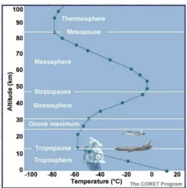
For the scope of this work, particular interest will be given to the influence of obstacles on urban climate and energy consumption in buildings. Urban climate and the evaluation of energy consumption inside buildings in urban areas depend on interactions between different spatio-temporal scales. To understand the pro- cesses which influence the urban climate, it is important to analyze the intricate behavior of the atmosphere. The Earth’s atmosphere is composed of four layers and is illustrated in Figure 2.1.

The troposphere contains about 80% of the atmospheric mass and most of the human activities and life are concentrated in this layer. The focus will hence be given only on the troposphere. The average height of the troposphere is about 10km (16 km at the Equator and 7km at the Poles). The troposphere can be further divided in the Planetary Boundary Layer (PBL) and the Free Atmosphere (see Figure 2.2).

The PBL is directly in contact with the Earth’s surface and responds to forc- ing from the land uses, the radiation and turbulence, as it will be explained in Section 2.2. The influence of surface friction and heating is transferred very effi- ciently to the PBL through turbulent mixing or transfer. These processes, which take place at different time and length scales, regulate the atmospheric circula- tions in the PBL. Close to the ground, a surface layer is developed. The Earth’s surface exerts a frictional resistance to atmospheric motions and slow them down [Arya,2001]. This surface layer is a region where turbulent fluxes and stress vary by less than 10% of their magnitude. This layer is also often referred to as the constant-flux layer.

However it is now generally acknowledged that this cannot be totally applied in urban areas [Roth, 2000]. The high density of vertical obstacles, the modification of the energy budget and wind patterns can lead to the formation of an additional

2-1

Figure 2.1: Structure of the Atmosphere (taken from www.ncsu.edu)

Figure 2.2: Planetary Boundary Layer

2.2 From the Global to the Building scale

Scale Length Time

Global > 500Km Years

Meso-scale 100-200Km Daily Neighborhood and street 1-2Km Hour(s)

Building < 100m <Hour

Table 2.1: Time and distance scale relative to the different spatial scales phenomenon called the Urban Heat Island. Particular attention will be given in this study to the processes taking place in the urban canopy and how they have been addressed in past studies.

Section 2.2 describes of the physical phenomena driving the weather/ climate at different scales (global, meso-scale, neighborhood and building). The interac- tions that exist between them is given in Section 2.3. The complexity and high heterogeneity of urban areas makes modeling an excellent tool to simulate the at- mospheric circulations as well as the energy use in these areas. A review of the state-of-the-art meso-scale and micro-scale models is made in Section 2.4 and the various processes that are taken into account at each of these scales are given.

Finally the limitations of these models will be pointed out and it will be explained how a canopy model can be used to overcome these limitations.

2.2 From the Global to the Building scale

Atmospheric processes are governed by processes taking place at different spatial scales. Each of these spatial scales are linked to a time scale through the wind velocity [Britter and Hanna,2003]. The relationship between the time and spatial scale can be expressed as follows:

x=ut (2.1)

where x is the spatial scale, u is the velocity andt is the time scale. Table 2.1 summarizes the four spatio-temporal scales which will be discussed in this section.

Britter and Hanna [2003] had an intermediate city scale which is omitted here, but is are included here in the meso-scale. Depending on the intended application,

2-3

more or less attention have been given by previous studies for each of these scales.

2.2.1 Global

At the global scale, the weather and climate processes are dominated by three main factors:

• The main driver for Earth’s climate is the Sun, more particularly the position of the Earth with respect to the Sun. The elliptic course of Earth around the sun and its rotation on itself as described by Galilei [1632, Ed. 2000], affects the global repartition of the incoming solar radiation which influences the atmospheric circulations on the entire globe.

• Earth’s climate is also highly influenced by the presence of greenhouse gases in its atmosphere. Over long periods of time (more than a year), the average temperature of the Earth can be considered constant [Ramanathan et al., 1992]. The presence of carbon dioxide and other gases (water vapor for example) causes the atmosphere to warm up as they absorb some of the energy that is emitted by the planet in the infra-red wavelength. This causes Earth’s average temperature to be around 15^◦C or 288K [IPCC, 2007].

• Other factors can also influence the Earth’s climate. For example, volcanic eruptions can release large amount of gases and small particles that can influence the energy budget of the Earth. Other climate-related events, such as the El-N˜ino, can also influence the atmospheric circulations for many years at various points on the globe.

Energy use inside buildings is thus mainly driven by the prevailing climate at a global scale since it will highly influence the climate at smaller scales.

2.2.2 Meso-scale

The meso-scale can be said to have a horizontal resolution of a few kilometers to several hundred of kilometers with a time scale of 1 to 24 hours.

2.2 From the Global to the Building scale

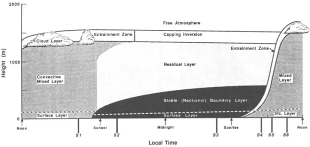
Figure 2.3: Evolution of the boundary layer during a diurnal cycle

At the meso-scale, a number of processes, along with the global variations, influences the atmospheric circulation. At this scale, complex topography, land- use characteristics, water bodies, atmospheric aerosols, snow, sea-ice and ocean interactions can have significant impact on the meso-scale atmospheric circulations.

Processes in the Planetary Boundary Layer become increasingly important for the atmospheric circulations. Figure2.3shows the evolution of the boundary layer during a diurnal cycle. The PBL, height and processes, evolves during the day and according to Stull [1988], the following description can be given for its evolution:

• The development of a mixed (convective) layer starts with the beginning of the day. Two situations contribute to the convection in this layer. Warm air rising from the surface creates thermals of warm air while cold air from cloud top sinks and creates thermals of cool air. The growth of this layer is entertained by the growing buoyant (heat-driven) turbulence which mixes it into the less turbulent air above the layer. The convective layer height varies in general between 1500m to 4000m.

• Just before sunset, the formation of the thermals stop and turbulence starts to dissipate without any more production. This layer does not have direct

2-5

contact with the ground, but pollutant, for example, can stay trapped in this layer since it originates from “former mixed layer”. This layer has thus been dubbed, the residual layer and is as such not part of the boundary layer.

• However under the influence of the ground, part of this residual layer is transformed at night in a stable boundary layer. The layer is characterized by weak turbulence. In such a layer, due to low vertical mixing, there is large horizontal dispersion, which can be seen, for example, with pollutants.

The planetary boundary layer is thus highly impacted by the land use. Large areas of vegetation, such as tropical forests, deserted areas, or urban areas can have a significant effect on the precipitation patterns [Lin et al., 2011] and the latent heat fluxes. Oke [1976] proposed that there is a distinction between the urban canopy layer and the boundary layer above it. A focus is given specially on how urban areas influence meteorological variables and circulation patterns around them.

Urban areas are made of a complex mosaic of land use and building forms.

These forms are characterized by a high density of vertical surfaces and are made of artificial materials. Urban areas induce thermal and dynamic effects that are quite different from a natural environment.

The specific thermal and radiative properties of materials used in urban areas for construction purposes (roads, car parks, houses, commercial areas...) differ from natural environment and hence urban areas tend to store more energy. The presence of urban areas also modifies the surface energy budget due to change in land use and the presence of vertical surfaces as compared to the surrounding areas. This tends to cause these areas to be warmer and temperature can increase by as much as 10^◦C [Santamouris et al.,2001,Chow and Roth,2006]. The presence of obstacles and the high density of vertical surfaces also generates a drag effect which modifies the wind patterns [Raupach, 1992, Martilli and Santiago, 2007, Hamdi and Masson, 2008, Aumond et al., 2013].

As the wind pattern and the atmospheric stability change on a daily basis, the atmospheric circulation inside urban areas is modified at the same scale (as opposed to the global scale whose time scales are quite large (years to thousands of years)). For example, at night, the atmosphere becomes very stable close to the

2.2 From the Global to the Building scale

Figure 2.4: Example of an idealized Urban Heat Island - Temperature profile above an urban area (taken from http://www.uta.edu)

surface (see Figure 2.3) and hence a new regime is developed. Both dynamic and thermal effects modify the surface temperature and can enhance buildings’ energy consumption for heating and cooling [Salamanca and Martilli, 2010, Santamouris et al., 2001].

The combination of all these effects generates a phenomenon which is referred to as an Urban Heat Island, which was first described by Luke Howard for a case study on London [Mills, 2008].

Below are a few of the physical reasons explaining the occurrence of this phe- nomenon:

1. Thermal Properties. Urban areas are built using man-made materials such as concrete and asphalt. These materials often have different thermal properties when compared to natural environment such as trees/forests. They have a distinctive specific heat capacity, thermal conductivity, albedo and emissivity [Oke,1982]. They thus modify the surface energy budget of a particular area, since they will absorb and re-emit differently. Urban materials usually tend to have a larger specific heat capacity which means that there will be a change in the sensible heat fluxes coming from the Earth’s surface as compared to vegetated environments. The heat released by the artificial materials at night is however trapped inside the urban areas due to the high density of vertical

2-7

surface (see next paragraph). This thus creates a distortion in the energy budget of the urban canopy layer and hence a temperature profile that is unlike that of the surrounding natural areas (see Figure2.4).

2. Building structures. The geometry of the buildings in urban areas has a great influence on the energy balance of cities and creates a particular temperature distribution over these areas. This is due to the fact that buildings can provide shade to the incoming solar radiation and also block the release of radiation back into the atmosphere depending on the sky view factor (a measure of the degree to which the sky is observed by the surrounding for a given point [Grimmond et al.,2001])[Arnfield,2003,Oke,1982]. Reflection of energy between surfaces is enhanced as well as energy absorption. The great density of high vertical surfaces further increases these effects in comparison to rural areas that are relatively flat. Longwave radiations emissions into the atmosphere are thus reduced while more short wave radiations are absorbed [Oke, 1982], hence leading to a disruption in the energy balance leading to higher temperature than surrounding areas [Arnfield,2003, Chow and Roth, 2006,Oke,1982,Santamouris et al., 2001].

3. Available humidity. Construction of buildings and roads requires the cutting down of trees and natural vegetation. The lack or absence of vegetation and water bodies in urban areas leads to the reduction of available humidity and of evapo-(transpi)ration [Oke, 1982]. A change in the latent heat fluxes inevitably contributes to the formation and enhancement of the Urban Heat Island, since the surface energy budget is modified. Evapo-(transpi)ration would normally act as a cooling agent whenever trees or vegetation are present and could help mitigate the effect of sudden heating [Taha, 1997].

4. Heat Generation. The presence of human population in metropolitan areas implies presence of buildings, cars, industries and so on. This leads to the use of energy for a variety of purposes such as cooling, heating and trans- portation. This is dubbed Anthropogenic Heat Generation. According to the IEA [2008], around 50% of the energy used in buildings (world energy use) were directly related to space heating/cooling. At mid and higher latitudes,

2.2 From the Global to the Building scale during winter, this also account for a significant part of the occurrence of the Urban Heat Island [Offerle et al., 2006]. In summer, the use of air con- ditioning system will contribute to the enhancement of Urban Heat Islands [Ohashi et al., 2007, Salamanca et al., 2011] which can in turn decrease the efficiency of air conditioning devices [Ashie et al., 1999].

5. Greenhouse gas emissions. Transportation, buildings and industries emit greenhouse gases from their energy consumption. Most of this energy pro- duced are used in urban areas. In France, for example, buildings only ac- count for about 23% of the emission of greenhouse gases, for 40% energy consumption. Local emissions of greenhouse gases and other air pollutants can enhance local warming [Oke et al., 1991, Oke, 1982] but more impor- tantly they affect the global climate. According to the IPCC, the global mean temperature would increase by as much as 6^◦C by 2100 and this could lead to an increase in the occurence of heat waves in urban areas, hence causing further distress to local population in these areas [IPCC, 2007].

6. Other factors. An increase in wind speed and cloud cover will tend to have a negative effect on the presence of Urban Heat Island [Arnfield, 2003]. How- ever, anti-cyclonic conditions, city size and population will tend to have a positive feedback on the Urban Heat Island intensity. This intensity is also increased at night and during summers. The presence of topographical fea- tures such as mountains can also impact the intensity of Urban Heat Island.

All these different factors contribute to make the temperature in cities around 3−10K higher than in rural areas [Oke, 1987]. One of the most dangerous and negative effects of the presence of an Urban Heat Island is the thermal comfort inside the city. Heat waves are enhanced and can lead to increased mortality like it was the case in France during the summer of 2003 [Poumadre et al., 2005, Fouillet et al., 2006]. However, it should be noted that the presence of an Urban Heat Island would lead to lower energy consumption during winter, particularly for high and mid-latitude countries, since cities tend to be warmer.

Since the population and activities inside cities are projected to increased in the future, an expansion of the urban areas and hence of the Urban Heat Islands can

2-9

be expected. This will thus lead to a rise in temperature during both summer and winter. While in winter this will cause the energy consumption linked to heating to drop (for high and mid-latitudes countries), in summer the energy consumption will escalate with the use of air conditioning. This will further be enhanced by the likelihood of more heat waves as mentioned by the Fourth Assessment Report of the IPCC on the impacts of global warming [IPCC, 2007].

To summarize, the meso-scale is affected by a number of factors (land cover, topography, global climate, ...). Flow above the urban canopy is disturbed and deflected, and is even sometimes visible with a capping cloud [Britter and Hanna, 2003]. Due to the variations of land uses in urban areas, there is an increase in the complexity of the weather processes in the planetary boundary layer. The time scale for processes driving the weather at this scale is relatively small (∼ day) as compared to the global scale (∼year(s)) while the spatial scale here is of the order of a couple of hundred of kilometers. It can thus be seen here that the macro-scale structure of the city can significantly influence the atmospheric circulations at the meso-scale in particular with regards to the the Urban Heat Island occurence.

2.2.3 Neighborhood and Street scale

At the neighborhood scale, the urban canopy interacts directly with the atmo- sphere and thus impacts directly the atmospheric circulations in the canopy. The spatial scale here varies from 1-2km. The flow can be assumed to be at quasi- equilibrium, and is a result of change from other scales [Britter and Hanna,2003].

Even though above the canopy the wind can correspond to a classical logarith- mic profile, the same thing is not necessarily true inside the urban canopy [Britter and Hanna, 2003, Kastner-Klein and Rotach, 2004] as the flow structure in the roughness sublayer is highly impacted by the morphological characteristics (height and size of buildings,...) of urban areas.

In this transition zone, the impact of urban areas on turbulence production is also enhanced [Rotach, 1993a,b,Kastner-Klein and Rotach, 2004].

Excess heat produced inside buildings is rejected in street canyons in urban areas. The flux exchanges between the urban canopy and the atmosphere are hence modified and can bring changes in the circulation patterns at a larger scale.

2.2 From the Global to the Building scale The presence of building or green areas at the neighborhood scale can also modify the wind and the temperature profiles [Park et al., 2012]. At the neighborhood level these changes occur at the time scale of an hour and thus can influence very rapidly the heat island and the atmospheric circulations.

2.2.4 Building scale

The horizontal spatial scale for this category is from a few meters to about one hundred meters and concern the lowest 5-10% of the PBL [Foken,2008]. The time scale for processes at this scale is of the order of the hour. People inside cities live at this particular scale and most of their activities (including emissions of pollutants) takes place here. One of the reason why processes at this scale drew attention, was to evaluate the dispersion of pollutants inside street canyons.

This scale is highly influenced by the roughness elements that are present such as buildings or plants. In the case of urban areas, the variation of building heights and density will impact this roughness length [Foken,2008].

For the scope of this study, exchange with the street canyon will be the main interest. The surface layer is the layer where the main energy exchange takes place (see Section2.1). Processes involved at this scale include solar energy transformed into other forms of energy and also the modification of wind patterns due to friction [Foken, 2008].

The heat coming from the surface will influence the production of turbulence since it will influence the atmospheric stability in the surface layer. The occupants of a building will use more or less energy inside buildings depending on the time of the day but this usage will also be influenced by the local heat exchanges. Buildings which are better equipped (e.g. better insulation) will tend to less disrupt less the atmospheric circulations at this scale.

Moreover, at this scale, mechanical turbulence is generated and enhanced by the presence of obstacles. The presence of obstacles generates a drag effect which modifies the wind patterns [Raupach, 1992, Martilli and Santiago, 2007, Hamdi and Masson,2008,Aumond et al.,2013] and hence have an effect on the wind flow.

Both of these effects will contribute as sources or sinks of heat and momentum within the street canyons. Thermal turbulence at this scale is small as compared

2-11

to the production of mechanical turbulence. This then induces changes that will impact the meteorological variables profiles in the urban canopy. In fine the in- tensity of the Urban Heat Island can be modified (e.g. on a calm day or stable night), simply with modifications taking place at this scale.

Besides, the surface layer turbulence is responsible for exchanges between the atmosphere and the Earth’s surface. The flow in the street canyon will also depend on the characteristics of the flow above [Britter and Hanna, 2003]. This is for example the case at night when there is a stable boundary layer.

2.3 Interactions and feedbacks

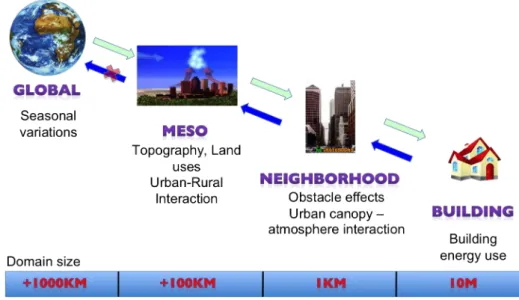
In Section2.2, the different scales were presented and it has been made clear that a number of processes influences each of these scales but, that there are strong interactions between each one of them. Figure 2.5 shows the chain of interactions that creates a feedback loop up from the building scale (micro-scale) to the scale of the city (meso-scale) to influence the intensity of a heat island above an urban area. The fact that building energy consumption depends on all the different scales highlights the importance of determining the impacts of buildings on the climate at the meso-scale level and vice-versa.

The global climate is driven essentially by the position of the Earth with respect to the Sun. The time scales at which these changes occur are larger than the time scales that are involved at the other three scales (meso-scale, neighborhood and building). Since the global scale has such a different time scale than the other ones, one can assume that there is no direct feedback on the global scale (although it is known that urban areas are responsible for an important part of greenhouse gases emissions - which in turn contribute to global climate change).

Previous studies have also suggested that Urban Heat Islands (or the presence of urban areas themselves) do not have a direct significant influence on the global climate or global temperature [IPCC, 2007, Parker, 2006]. However a few recent studies have shown that it is not to be totally neglected at the global scale [Mah- mood et al., 2013]. A recent study also suggested that energy consumption at meso-scale can influence, on a relatively short time scale, the global climate and there can be disruption or changes in global wind circulations [Zhang et al.,2013].

2.3 Interactions and feedbacks

Figure 2.5: Multi-scale climate interactions (Global scale to micro-scale)

Assuming that this is not the case, the following chain of action and interac- tions can be proposed. Changes in the global climate are essentially driven by the Sun and hence are seasonal or yearly. It thus influences the meso-scale atmo- spheric circulations. At this scale, the land use becomes increasingly important and the presence of urban areas, the modification of the energy budget and wind circulation, cause the development of an Urban Heat Island. This, in turn, will impact the weather processes in the urban canopy which then interacts with the buildings. The energy consumption inside buildings within urban areas is regu- lated by all these processes. The buildings themselves will release heat inside the urban canopy and will also have an impact on the circulation pattern at the neigh- borhood scale. In this transition zone, the buildings’ top will also be responsible for an increase in turbulence at this scale. The modifications brought at the urban canopy scale will then impact the weather processes at the meso-scale level, influ- encing again the intensity of the Urban Heat Island. As atmospheric circulations, and not climate processes, are the main goal of this study, it can be assumed on small time scales that there is no feedback to the global scale. Figure2.6 show the different processes and interactions between the meso- and micro-scales.

2-13

Figure 2.6: Interactions between the meso-scale and building (micro-scale) (Voogt, 2007)

2.4 Models

As it was seen in Section2.3, urban meteorology and the occurrence of Urban Heat Islands are the result of very complex non-linear physical processes and can cause a number of environmental disturbances. A lot of progress has been made during the last decades in this particular field particularly regarding weather forecast at the urban scale [Baklanov et al., 2002, 2005]. But there is still a lack of models that can grasp the whole extent of urban processes that influence the intensity of Urban Heat Islands.

It would be unrealistic to try to represent the complete heterogeneous nature of urban areas due to the limited CPU power and data availability [Martilli,2007].

However, there have been several attempts, using various techniques, to under- stand the processes that regulate the climate around a metropolitan area. At first, observations of the surface energy budget were used to build empirical models [Grimmond and Oke, 1999]. These models were just as realistic as the data that

2.4 Models were obtained through intensive measurement campaigns. Results were obtained using statistical tools to reproduce the existing conditions. Nevertheless, these models could only be used under the same conditions in which the measurements were made and could not be applied in cities with different situations.

This hence highlighted the importance of more physically-based numerical modeling. Since it was not possible to reproduce an urban area to the finer details, it was proposed that only the basic structures of cities were considered. Below, a description of models at the meso-scale as well as models at the building scale are given. Most models at the meso-scale that have been developed were used to evaluate the impact of urban areas and land use changes on the weather at this scale and on pollutant dispersion. Models at the building scale that are given here were used to calculate and represent the impacts of buildings on the energy use inside these buildings. These descriptions will show how the processes described in Section 2.2are taken into account in these models, and hence how realistic they are. The differences between the models will also be shown.

2.4.1 Meso-scale models

As mentioned in Section 2.2, the horizontal scale of the meso-scale varies from a few to hundred of kilometers with a time range varying from hours to a day. The smallest scale matches with atmospheric features for weather forecasting whose characteristics can be represented statistically, while the longer limits correspond to the smallest features which can be seen at a synoptic scale [Pielke,2002].

The horizontal domain size is sufficiently big to make the hydrostatic approxi- mation, but is too small for geostrophic wind to be an appropriate approximation in the Planetary Boundary Layer. The resolution that is used at this scale also depends on the computer performance [Martilli, 2007].

Meso-scale models working at this scale have been designed to take a number of processes, specially in urban areas, into account. Several models have been de- veloped in the recent years including NIRE-MM [Kondo,1989], MM5 [Grell et al., 1994], FVM [Clappier et al., 1996], MESO-NH [Lafore et al., 1997] or WRF [Ska- marock et al., 2008]. Each model was developed for several functions: (1) opera- tional forecast models or (2) for dispersion or (3) to evaluate the thermal energy

2-15

budget of urban areas or (4) for other research purposes.

For the current study, focus is given on the impact of urban areas on meso-scale meteorology. In this context, the following processes are known to be taken into account in these models:

Vertical Processes Each of the model reproduces the generation of the sur- face layer (see Figure 2.2). This means that they include a calculation of the solar radiation and are able to calculate the production of mechanical and thermal (buoyant) turbulence. Some of them, such as WRF, include cloud formation which can also influence the occurrence or the intensity of Urban Heat Islands.

Horizontal Processes The formation of an Urban Heat Island is also rep- resented in these meso-scale models. This would mean that they have been able to take into account the interactions that can exist between the rural and urban areas at these scales. To do so, these models should be able to modify the energy budget in urban areas as compared to a natural environment, and also modify the wind profile, which show that the model should be capable of accounting for more complex land use. Modification of wind pattern at this scale also arises due to the interaction between rural and urban areas, highlighting the need for large domains where advection processes can take place.

According toBaklanov et al.[2005], two types of approaches have been adopted in the past to calculate the influence of urban areas in meso-scale meteorological models:

• Monin-Obhukov Similarity Theory (MOST)The MOST developed byMonin and Obukhov[1954] and adapted by Businger et al.[1971] andZilitinkevich and Esau [2007], was mainly applied for non-urban surfaces. It is modified by using new values for the roughness length, displacement height and heat fluxes. The first model level is generally displaced at the top of the canopy (displacement height). The main disadvantage of such models is that they cannot take into account the high heterogeneity of urban areas. Roth [2000]

argued that the MOST does not hold in urban areas, and according toArya

2.4 Models [2005] the similarity theories can only be applied over homogeneous surfaces.

New diagnostic analytical models have thus been developed for the urban roughness layer to modify the calculation of the meteorological variables [Baklanov et al., 2005].

• Urban parameterization In these types of models, new sources and sinks terms, for each of the variables (momentum, heat and turbulent kinetic en- ergy), representing building effects are calculated [Masson, 2000, Kusaka et al., 2001, Martilli et al., 2002]. These parameterizations calculate the mean thermal and dynamic effect of urban areas on the atmosphere [Sala- manca et al.,2011].

A focus is given here on urban parameterizations as they are more pertinent to this study. With increasing computer performance, simplified parameterizations of cities were introduced in urban models coupled with atmospheric models to under- stand its impact on the boundary layer as well as the meteorological variables. In these models, the buildings and urban areas were simply represented as porosities.

The first generation of models, that included urban parameterization did not take into account the vertical surfaces present in urban areas. Their primary goal was essentially to modelize the modification of the energy budget of urban areas [Grimmond and Oke, 1999].

In a second attempt, the buildings were represented as uniform cubes that were regularly spaced [Kikegawa et al.,2003], so as to take into account the high density of vertical surfaces, which influence the energy budget of the city.

Furthermore two other types of models were developed and gave rise to more complete parameterization schemes. Both schemes solved the energy budget in a 3- dimensional urban canopy where buildings are represented with a basic geometry.

Urban areas have a variety of surfaces that are exposed to radiation (roof, wall and streets) and those surfaces radiate part of the energy they receive back into the canopy layer. In addition, these models also take into account the influence of buildings or obstacles on the wind circulation pattern via a drag-force approach.

The main difference between these two schemes is that in one the urban canopy layer can be immersed in several vertical layers of the meteorological model (hence multi-layer)[Kondo and Liu, 1998, Kondo et al., 1999, Ca et al., 1999, Martilli

2-17

Figure 2.7: Representation of the urban canopy: left: single layer and right: multi- layer

et al., 2002] while for the other the canopy layer is forced from data coming from the first meteorological layer[Kusaka and M., 1999, Kusaka et al., 2001, Masson, 2000]. This is illustrated in the Figure2.7.

Another difference between some of the models is that some do not take into account the orientation of the canyon and hence there can be discrepancies in the energy budget that is calculated at this scale and that is received by the buildings [Kusaka et al.,2001].

Previous works were carried out to improve the calculations of the fluxes that feedback on the meteorological model. A Finite Volume Method model (FVM), developed by Clappier et al. [1996], has been used to make such developments.

Martilli et al. [2002] worked on the source terms from the surface while Rasheed [2009] worked on the diffusion processes in the urban canopy. Krpo [2009] de- veloped a Building Energy Model (BEM), which was coupled with FVM, and Salamanca et al.[2010],Salamanca and Martilli[2010] showed that BEM is highly influenced by the weather processes at this scale.

Table 2.2 shows a selection of urban canopy parameterizations that have been implemented in meso-scale models as well as some of the characteristics of these models. Salamanca et al. [2011] compared the different schemes (Bulk, UCM, Building Effect Parameterization (BEP) and BEP-Building Energy Model) and showed that depending on the use for the meso-scale model, the appropriate scheme should be then chosen.

As it was mentioned in Section 2.2, a number of different factors affects the in- tensity of Urban Heat Islands. Depending on the use of the model, several schemes have been adopted and validated. For numerical weather prediction at this scale,

2.4Models

Model Authors Resolution of

canopy

Vegetation Primary use Anthropogenic heat

MM5 MRF BL Liu et al. [2006] No canopy, roughness length modification

No Weather Fore-

cast

No

ARPS Sarkar and De Rid-

der [2011]

Yes UHI formation Yes

Meso-NH-TEB Masson [2000] Single layer Yes Urban meteorol-

ogy

from fixed tem- poral files

Kusaka et al.[2001] Yes Yes

SUMM Kanda et al. [2005] Yes No

FVM-BEP Martilli et al.[2002] Multi-layer Yes Air pollution modeling

No

WRF-BEP Yes No

NIRE-M Kondo et al. [2005] Yes No

MM-CM-BEM Kikegawa et al.

[2003]

Multi-layer Yes Building energy

use, air pollution modeling and urban planning

Yes

WRF-BEP-BEM Salamanca et al.

[2010]

Yes Yes

Table 2.2: Urban canopy parameterization implemented in meso-scale models (adapted fromSalamanca et al.[2011])

2-19

Figure 2.8: Grid in a meso-scale model

simple urban parameterization can grasp Urban Heat Island generation and be used to forecast at this scale. For other needs, such as pollutant dispersion or energy budget of urban areas, more complex parameterizations have been devel- oped [Salamanca et al.,2011]. These parameterizations have shown that they are able to reproduce the effect of urban areas on the planetary boundary layer. Even though these parameterizations are really powerful now and have been able to represent the interactions between the urban areas and the atmosphere, buildings and streets are still not ‘seen’ in the grid cells of the meso-scale models due to the low vertical and horizontal resolution (see Figure 2.8). To be able to achieve this, an increase in the vertical and horizontal resolution would be needed and this would require tremendous amount of computational time and data collection.

2.4.2 Micro-scale models

A series of micro-scale models have been developed in the recent decades. Each has been used in different configurations and thus have different capabilities (air pollu- tion problem, vegetation, building energy use, ...). In the present work, the focus will be given mainly to models used in the evaluation of energy use in buildings.

The processes driving the meteorology at the micro-scale is limited by phe- nomena which originate from the surface layer of the Planeteray Boundary Layer

2.4 Models

Figure 2.9: Grid in a micro-scale model

[Arya,2001] and which are essentially influenced by the frictional forces,.

In micro-scale models obstacles are not represented like porosities. Buildings, roads and other obstacles can be explicitly described(see Figure2.9) in these mod- els which allow for precise calculations of the variables (momentum, energy and turbulent fluxes and energy consumption).

Standard E-ǫ(turbulent kinetic energy - dissipation) closure models and Navier- Stokes equation are usually used to resolve the turbulence and variables respec- tively [Yang et al., 2013]. Sources or sinks, for the momemtum, energy (heat) or humidity, are calculated and impact each of these variables. These models take into account the following processes:

Mechanical Effect At these scales, as it was shown in Section2.2, mechanical effect of the buildings or obstacles are an important source of perturbation of the atmospheric circulations. These obstacles will modify the wind and temperature profiles and will generate turbulence. Micro-scale models can thus calculate the impact of the obstacles, often parameterized using a drag-force approach, on the wind flow.

Thermal Effect Some of the micro-scale models have been developed to ac- count for the thermal effect (change in radiation). In these models, the height to

2-21

which an air parcel can travel, can be as high as the PBL, due to the convection processes that can be initiated. Such models can also differentiate between hu- mid and dry convection which can influence the latent heat fluxes, crucial for the dissipation of heat.

Some micro-scale models such as Envimet [Bruse and Fleer, 1998] use a prog- nostic equation to calculate the evolution of the variables. These models can reproduce a more typical climate at this scale than steady-state simulations which can only simulate for small period of time [Bruse and Fleer, 1998]. Micro-scale model can receive their hourly data either from other meso-scale model or from a database where they can extract an average dataset for a particular location.

Table 2.3 shows a selection of micro-scale models used to simulate energy bal- ance and used in urban areas. A more complete description of building energy use models can be found in Crawley et al. [2008].

2.5 Limits of e