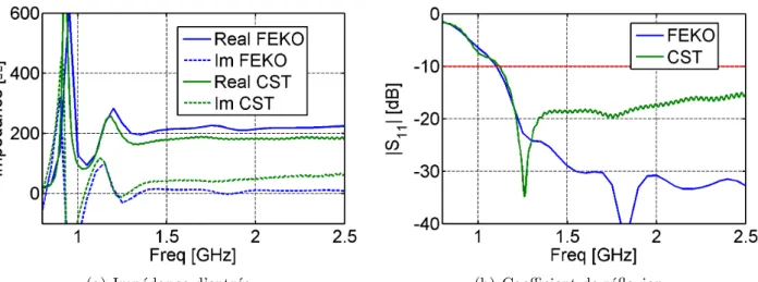
5 montre l'impédance d'entrée et le coefficient de réflexion pour l'antenne de la Fig. Le calcul du champ électrique total d'un réseau d'antennes nécessite la solution exacte de la.
Introduction
Antenna basics
Some antenna concepts and definitions
Another common indicator of the AR is the Cross Polarization Rejection (XpolR), usually expressed in dB. The direction of the antenna (D) is the power density in a certain direction versus the average power density created by the antenna.

Broadband antennas
The gain of an antenna (G) is the ratio between the power delivered by the antenna in a certain direction versus the power delivered to the antenna. The direction will always be greater than the gain since the latter includes the losses, such as losses in the substrate, losses due to charges in the antennas, etc. If the gain of the antenna reaches this value, it is said to have a 100% aperture efficiency.
With the addition of ridges, this antenna can be bilinearly polarized and its bandwidth can increase to 15.7:1 of bandwidth (Van der Merwe et al., 2012) (cf. For applications in the air, planar structures have certain advantages, such as the possibility of being mounted in the skin of an aircraft.
The Archimedean spiral antenna
- Type of spirals
- Feeding system
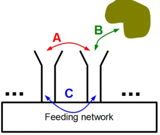
- Cavity
- Miniaturization
This difference is again due to the reflected currents, as in the case of the impedance matching. Making the coil operate at frequencies below this frequency is the goal of the miniaturization. It slows down the current speed in the arm of the spiral and adds reactive components, like in a transmission line.
It also allows for an easier way to adjust the spiral antenna by changing the characteristic impedance of the spiral's arms. The main idea is to introduce an inductive load using the shape of the spiral arm. When resistive loads are placed at the end of the coil's arm, the current is absorbed.

Antenna array basics
- Mutual coupling
- Array factor
- Uniformly spaced arrays
- Non-uniformly spaced arrays
- Dual polarization capability
- Array bandwidth
Changing the excitation of the antennas, as in the case of beamforming, will change the induced. In addition, we can define the position function of the elements in relation to the wavelength, as in Eq. From this we can derive the condition to avoid the presence of the maximum of the lattice lobes (in this case the first one, m = 1) in the "visible region" (Mailloux, 2005):.
In fact, the Fourier transform of the x-y array lattice, divided by λ, is its lattice reciprocal in u-v space (Kittel, 1995). We have shown that the grating of the array plays an important role in the presence of the grating lobes and the side loop levels. In these cases, the coupling between the elements can increase or decrease the bandwidth of the array.
Summary of chapter
We have considered the cases of waves perpendicular and parallel to the plane of the spiral. We can see that a transmission line pattern is formed between the arms of the coil. Therefore, the group cutoff frequency is approximately the same as in the case of a single square coil (0.92 GHz).
Linear Array of Spiral Antennas
Introduction
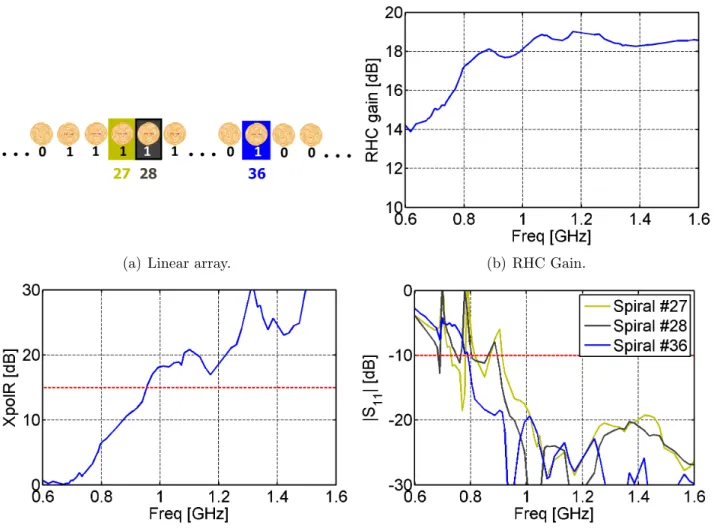
The next step is the study of mono-polarized linear arrays composed of helical antennas where, due to mutual coupling, several problems arise.
Resonances in a linear array
- An example of a linear array
- Standing waves found in just one spiral
- Explanation using transmission line theory
- Solutions
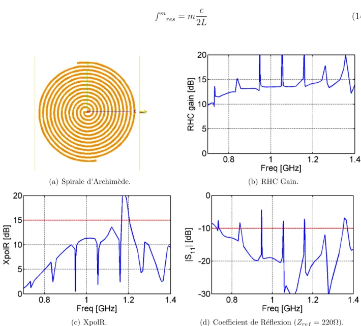
These resonances are related to the length of the arms of the helix according to Eq. The zero point in the center of the spiral reveals that the current does not reach the center. Only the second wave, with direction parallel to the plane of the spiral, induces a strong standing wave in the arm of the spiral.
This wave can be decomposed into two waves with directions perpendicular and parallel to the plane of the spiral. On the other hand, the wave with direction parallel to the plane of the spiral will induce mode 0. The phase difference in the middle of the spiral is then approximately 140◦ and not 0◦ as in Fig.

Mono-polarized uniform linear array
- Analytical estimation of the bandwidth of linear arrays
- Simulation of linear arrays of asymmetrical spirals
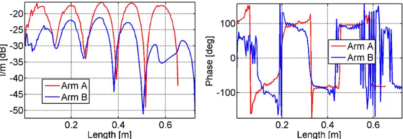
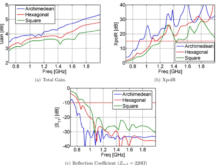
By doing this, we obtain good impedance matching, but the circular polarization is not really improved, as can be seen in the results of the linear array of asymmetric helical antennas in Fig. The circular polarization of the array is acceptable for frequencies higher than 1.24 GHz, while for a single spiral it was 1.21 GHz. We see a peak at 0.73 GHz in the reflection coefficient, which corresponds to the Steyskal resonance of the smaller arm.
The cutoff frequency of the XpolR is 1.12 GHz, while for a single coil it is 1.07 GHz. BWS11 and BWXpolRa are the bandwidths of the arrays using the reflection coefficient and rejection of cross polarization cutoff frequencies and grating lobe frequencies, respectively. 2.9 we can see that, for the case of S11 bandwidths, only the sequence of asymmetric Archimedean spirals reaches the analytical limit of the bandwidth.
Dual polarized linear array
This is so because, at higher frequencies, the radiation zone gets closer to the center, so the current does not reach the outer parts of the arms which lowers the coupling, unlike what happens at low frequencies. For the rest of the spirals, the reflection coefficient becomes acceptable for frequencies higher than 0.81 GHz. Since only 2 spirals out of 40 have problems for each polarization, we can see that there are no peaks in the XpolR and gain of the array, in contrast to the case of uniform linear arrays where the peaks are also present in the XpolR and gain.
Summary of chapter
The introduction of spirals of opposite polarization, to obtain a dual polarized array, reduces the bandwidth of the array. This will lead us to improve the lower limit of the bandwidth of the array. The simplest case is the design of a planar series of spirals of the same polarization in a uniform grid.
This time the grid lobes of the bandwidths for a square grid in Eq. In this array, the equation for the grid lobes is the same as in the case of the Archimedean spirals in a triangular grid (cf. The distance between the bottom of the cavity and the spirals was also kept at 5 cm.
Planar Array of Spiral Antennas
Introduction
Using uniform arrays and for the case of mono polarization, the bandwidth of linear arrays of spirals cannot exceed one octave for the maximum scan angle θ = 30◦ . So far, only the broadband array design trend focusing on the use of broadband antennas has been considered. In the first part of this chapter, we will again follow the first design trend.
Then we will work with non-uniform arrays, concentric ring arrays, which will help us improve the highest bandwidth limit. By combining the two design trends, we will achieve a very large bandwidth operating with two opposite polarizations.
Mono polarized planar array of spiral antennas
- An example of a mono polarized planar array of spiral antennas 67
- Simulations of planar arrays to validate analytical method
- WAVES technique in uniform planar arrays
XpolR is not good in the green range and this is due to D determining the lowest cutoff frequency of the array's bandwidth. The bandwidths are then calculated using the "p" factor of the coils, for the lowest cutoff frequency (cf. The XpolR lowest cutoff frequency of the array (0.88 GHz) is approximately the same as that of a single coil of this size (0.9 GHz).
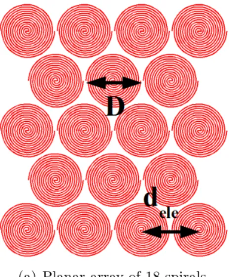
The results show that the lowest cutoff frequency of XpolR is slightly larger than that of S11. Again, the lowest cutoff frequency for XpolR is 0.89 GHz, which corresponds to a single helix. We will maximize the total bandwidth of the array of Archimdean spiral antennas with two sizes in an equilateral triangular array sketched in Fig.
Dual polarized planar array (6:1 bandwidth)
- Design and measurements of one ring array
- Applying first design trend: Adding more rings
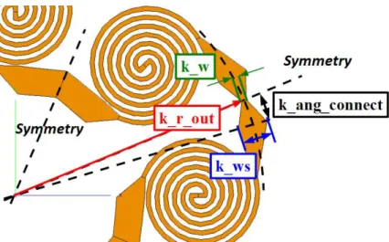
- Applying second design trend: Connecting the spirals
In the case of the array, the reflection coefficient improvement is due to the presence of the cavity and the coupling with the other coils. But the array cavity also affects the input impedance of the coil, increasing the reflection coefficient slightly more than -10 dB at 1.35 GHz and 2.1 GHz. This problem can be overcome by optimizing the alignment of the element in the cavity and the feeding system.
In fact, we can see that the reflection coefficient of the spiral with substrate starts a little earlier. In order to speed up the optimization process, the substrate of the spirals was not considered. At the time of writing this work, the measurements of the one ring array with the optimized connections are performed.

Summary of chapter
Using non-uniform arrays does not affect the XpolR of the array or its efficiency. Mastoris (1981), Polarization dependence in electromagnetic inverse problems, IEEE Trans. 2009), Polarization constraints in bipolarized phased arrays derived from an infinite current blade model, IEEE Antennas Wireless Propag. Vigano (2011), A new deterministic synthesis technique for constrained sparse array design problems, IEEE Trans. 2001), Star spiral design and analysis with application to variable element size broadband arrays, Ph.D.
Vouvakis (2012), The flat ultra-wideband modular antenna (puma) array, IEEE Trans. 2007), Dual Polarized Broadband Array Antenna with Boron Elements, Mechanical Design and Measurements, IEEE Trans. Chang (2006), A multiband, compact, and full-duplex beam-scanning antenna transceiver system operating from 10 to 35 GHz, IEEE Trans. 1986), An array technique to generate circular polarization with linearly polarized elements, IEEE Trans. Steyskal (2009), Analysis and power supply of a spiral element used in a planar array, IEEE Trans. 1965), simple relations derived from a phased array antenna made from an infinite current blade, IEEE Trans.
Conclusion
Conclusion
The analyzes and examples of different cases of uniform linear arrays led us to a better understanding of the resonance issues presented in uniform arrays of helical antennas. If we want to design a dual-polarized array using two-armed coil antennas, we must use coils with opposite polarization, which means that the distance between the elements of the same polarization will be greater. The larger distance is synonymous with the appearance of the grating lobes closer to the broad direction.
Concentric ring arrays allowed us to also use the connecting spiral technique, which improved the lower bandwidth limit of the array. The presence of grid lobes is related to the minimum distance between the sources, but the size of the antenna limits this distance. This means that the curvature of the surface over which the spirals are positioned will help to slow down the presence of grid lobes.