is a multi-disciplinary open access archive for the deposit and dissemination of sci- entific research documents, whether they are pub-

(1)

HAL Id: inria-00151600

https://hal.inria.fr/inria-00151600v1

Submitted on 4 Jun 2007 (v1), last revised 7 Jun 2007 (v2)

HAL

is a multi-disciplinary open access archive for the deposit and dissemination of sci- entific research documents, whether they are pub-

L’archive ouverte pluridisciplinaire

HAL, est

destinée au dépôt et à la diffusion de documents scientifiques de niveau recherche, publiés ou non,

Axisymmetric Reflector Antennas

Benoît Chaigne, Jean-Antoine Desideri

To cite this version:

Benoît Chaigne, Jean-Antoine Desideri. Parametric Shape Optimization for the Conformation of

Axisymmetric Reflector Antennas. [Research Report] 2007, pp.27. �inria-00151600v1�

(2)

a p p o r t

d e r e c h e r c h e

ISRNINRIA/RR--????--FR+ENG

Thème NUM

Parametric Shape Optimization for the

Conformation of Axisymmetric Reflector Antennas

Benoît Chaigne — Jean-Antoine Désidéri

N° ????

Septembre 2006

(3)

(4)

Benoît Chaigne

^∗

, Jean-Antoine Désidéri

^∗

Thème NUM — Systèmes numériques Projet Opale

Rapport de recherche n°???? — Septembre 2006 — 27 pages

Abstract: A shape reconstruction problem of axisymmetric radiating structures is considered. This reads as an inverse problem. The direct problem - expression of the electric field w.r.t. a given geometry - is approximated by a simple model. For the inverse problem - find the shape whose radiation has been measured - a parametric shape functional is defined for which the Free-Form Deformation method is introduced. Two different strategies to solve numerically the inverse problem (minimize the functional) is discussed: the first one is deterministic and the other one semi-stochastic. It appears that the functional is highly multimodal. At last, a multilevel strategy is proposed for which we discuss both robustness and convergence.

Key-words: inverse problem ; shape optimization ; Free-Form Deformation ; Particle Swarm Optimization ; multilevel methods ; electromagnetics ; reflector antenna ; radiation diagram

∗INRIA Sophia-Antipolis, OPALE Team

(5)

Résumé : On considère un problème de reconstruction de forme de structures rayonnantes axisymétriques. Il s’exprime comme un problème inverse. Le problème direct - expression du champ électrique en fonction d’une géométrie donnée - est modélisé par une formule approchée. Pour le problème inverse - retrouver la forme dont le rayonnement a été mesuré - une fonctionnelle de forme est définie paramétriquement. À ce propos la méthodeFree- Form Deformation est introduite. Nous comparons alors deux stratégies différentes pour résoudre numériquement le problème inverse (minimiser la fonctionnelle) : une déterministe et une semi-stochastique. On montre à cette occasion le caractère multimodal de la fonctionnelle. Enfin, à la vue des résultats, on propose une méthode hiérarchique afin d’améliorer la robustesse et la convergence.

Mots-clés : problème inverse ; optimisation de forme ; Free-Form Deformation ; optimisation par essaim de particules ; méthodes multi-niveaux ; électromagnétisme ; antenne à réflecteur ; diagramme de rayonnement

(6)

1 Introduction

Antenna conformation is a real-world electromagnetic issue that arises each time a reflector antenna is designed. For instance the radiation of the antenna should cover a specific geographical area while avoiding others, under international norms. Or it should keep ideal properties considering the influence of the structure that hold it.

Practically, it often requires physical intuition from conceptors. However this problem can be defined as an inverse problem yielding a shape optimization problem [5, 6]. In some special cases this problem reads as a shape reconstruction problem for which there are successful methods [6] involving multilpe frequencies.

The study aims to explain why the problem is hard to solve and then suggests new methods for solving it. First, the equations for the direct problem are recalled. Then the shape parameterization is introduced, which can be critical in such problems. In an other part the objective functional of the inverse problem is defined. At last a case study is conducted where different strategies to reduce the objective function are compared.

2 Direct problem: computing the electric field

A reflector antenna in transmission is composed of a source of electromagnetic (EM) waves and a reflector considered as a conductor object (see Figures 1 and 2). Physically, the source will induce surface currents onto the reflector which will then act as a secondary EM waves source. The direct problem consists in determining the resulting electric field in a domain Ω, considering a geometry and an incident wave.

Electromagnetic phenomena are modeled by Maxwell equations [1, 3]. However, a simpler model known asphysical optics, well suited for the problem, will be considered. This model, for which the electric field becomes explicit w.r.t the geometry, allows us to avoid the heavy computations of using a Finite Element solver.

In this study axisymmetric reflectors and a single monochromatic source are considered.

More precisely, the diameter of the aperture is around 30 cm, thus a reasonable frequency is f = 10GHz. The wave velocityc is equal to the speed of light in vacuum and thus the wave length isλ=_f^c = 2.99792458·10⁻²m, that is, one tenth of the aperture.

2.1 Expression for the electric field, Physical Optics model

As said previously the Maxwell equations describe the EM field(E, ~~ H). The directive gain, which will be introduced in section 2.2, involves the far field power for which the electric field will be sufficient. Therefore one focuses on E. Physics about EM field and antennas~ can be found in [1, 3].

Let O be the source localization and S the reflector surface. The total electric field E~ at a pointP results from the summation of the incident fieldE~ⁱradiated by the source and the scattered fieldE~^s:

E(P~ ) =E~ⁱ(P) +E~^s(P). (1)

(8)

Figure 1: example of a toroidal reflector antenna with several sources [4]

IfP, identified byR~=−−→

OP, is far enough from the reflector (far field) and if the diameter of the reflector is much larger thanλthe scattered field is given by:

E~^s(P) =−iωµe^−ikR 4πR

Z Z

S

hI~− I~·R~

R~i

e^ikρ(^R·~^~^ρ)dS, (2) whereµstands for the magnetic permeability,ωthe wave pulsation andkthe wave number (k= ^2π_λ). I~is the induced current onS at a pointQidentified in (2) by~ρ=−−→

OQ.

Thephysical opticsapproach consists in considering that at each point of the surface, the scattered wave is equivalent to the scattered wave on the tangent plane, perfectly conductor.

This means in particular that the diffraction effects due to singularities on the reflector (such as the border) are neglicted. This model is quite accurate when the wave length is much smaller than the reflector, as assumed. Thus, formally, the surface current onSis given by:

I~=−2~n×H~ⁱ, (3)

whereH~ⁱ is the incident magnetic field.

2.2 Directive gain

The directive gain is the radiation intensity (power radiated by unit solid angle) normalized by the one of the corresponding isotropic source [3]. The set of directive gain for a set of directions is called radiation diagram.

(9)

Figure 2: schematic scattering of a reflector antenna (parabola) [4]

Let U(θ, φ) be the radiation intensity for the (θ, φ) direction. In our case the power density is given by the Poynting vector:

P= 1

2|E~×H~^∗|= 1

2η|E|~². (4)

ThusU =R²P. In far fieldE~ is a spherical wave, which yields E(P~ ) =e^−ikR

4πR E(θ, ϕ).~ Consequently

U(θ, ϕ) = 1

2η(4π)²|E(θ, ϕ)|~ ². (5) Finally, to obtain the directive gain D, one must normalize with the intensity of the corresponding isotropic source which is the mean ofU over all solid angles, that is:

Ui= RR

ΩU(θ, ϕ)dΩ

4π , (6)

and hence

D(θ, ϕ) = U(θ, ϕ) Ui

= 4π|E(θ, ϕ)|~ ² RR

Ω|E(θ, ϕ)|~ ²dΩ. (7)

2.3 Numerical computation of the directive gain

Practically, for the computation of the radiation diagram, the considered source will be an elementary dipole for which the radiation(E~ⁱ, ~Hⁱ) is known analytically. It can be shown

(10)

that such a dipole is unimodal (in the sense that its Fourier serie decomposition reduces to a single modem= 1). Thus the knowledge ofE~ on the planes defined byϕ= 0andϕ= ^π₂ (forθ∈ [0,2π]) is sufficient to deduce the electric field everywhere else. Moreover, it can be shown that on each plane, only a single component (in spherical coordinates) is non zero.

The unknown, depending on a surfaceS, will from now be noted E(S, θ) =~

E^θ(S, θ) E^ϕ(S, θ)

(8) whereE^θ andE^ϕ stand for the non zero components.

The reflector being axisymmetric,Sresults from the revolution of a curveCofR²called meridian. Equation (2) reduces then to a single integral overC. Numerically,C is piecewise linear and the total scattered field corresponds to the sum of fields scattered by each segment.

The integrals over the segments are computed by Gauss quadratures.

0 0.5 1 1.5 2 2.5 3

theta (rad)

-80 -70 -60 -50 -40 -30 -20 -10 0 10 20 30

Directivity (db)

Diagram

0 0.02 0.04 0.06 0.08 0.1 z(t)

0 0.05 0.1 0.15 0.2

x(t)

source

Meridian

C

zc

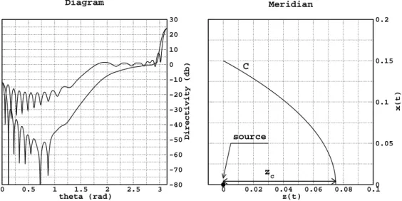
Figure 3: radiation diagram of a parabola radiated by an elementary dipole, f = 10GHz (λ= 30mm), aperture diameterd= 30cm= 10λ,zc= 7.5cm= 2.5λ

3 Parametric representation of the geometry

Parameterization was said to be critical in the introduction. Indeed, the choice of parameters will induce the nature of the optimization parameters. For instance, in [5] they are the nodes of discretization of the shape. The disadvantage of using such a parameterization is that singularities may be introduced during the optimization process. Moreover, it

(11)

introduces stiffness since the number of nodes should be large so that the direct problem becomes accurate enough. Therefore here is proposed an other parameterization where the optimization variables and the discretization are independant.

LetC be the meridian ofS represented in the half-plane as follows:

C

x(s)∈ C¹([0,1],R⁺)

z(s)∈ C¹([0,1],R) s∈[0,1]. (9) Note thatCshould be regular enough for thePhysical Opticsmodel to be valid. The surface S is obtained by rotation around the axis of equation x = 0. In addition the following condition is required:

x(0) = 0

z(0) =zc , (10)

wherezc represents the distance between the source (located at the origin of the system of coordinates) and the center of the reflector fixed on thez-axis (see Figures 3 and 4).

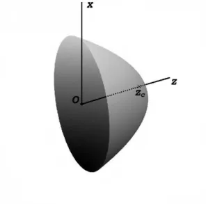
Figure 4: Paraboloid

The surface considered in the optimization will actually result from the deformation of an initial surfaceS⁰, namely:

S =S⁰+ ∆S, (11)

where ∆S, the deformation, depends on a finite number of parameters. This approach is known asFree-Form Deformation (FFD) method, first introduced for Computer Graphics issues [7], in order to deform 2D or 3D objects regardless of what these objects are (noted

(12)

S⁰ here). In this way the number of parametric variables, also called design variables, is chosen according to the parameterization. In addition, the smoothness of the shape will be controled as explained in 3.1

3.1 Free-Form Deformation principles

This section is devoted to explain theFFD technique for a 2D problem. LetCbe a curve of R²(non necessarily regular) contained in a subsetD⊂R². Considerφan homeomorphism that mapsD onto the unit square:

φ: D −→ [0,1]×[0,1]

(x, z) 7−→ (tx, tz)

, (12)

that is, a local system of coordinates on D is defined. Then, let {bk}ⁿ_k=1 be a linearly independent family ofR-valuedC¹ functions defined on[0,1]×[0,1]. The deformation of the domain D is then defined as a linear combination of the basis functions bk. Note that this approach defines a global smooth transformation over the whole domain. Formally, for all points(x, z)ofD,a fortiori ofC, the deformation reads:

∆x

∆z

= Xn

k=1

bk(φ(x, z))~pk, (13)

where~pk ∈R²,k= 1, . . . , n, are the coefficients of the deformation in the basis{bk}ⁿ_k=1. The spaceX≡span{b1, b2, . . . , bn}can be considered as the deformation space, which contains all the shapes that can be generated. Henceforth let~pkbe called the shape parameters. Since the parameterization applies on the deformation and not no the shape itself, no regularity ofC is required. Moreover, since the deformation is smooth, the singularities are kept.

Theoretically any (linearly independent) family {bk}ⁿ_k=1 can be considered. Practically, in this study and historically [7], a tensorial product of Bernstein polynomials is used. This is justified by certain of their properties that will be discussed in the next section. The deformation reads then as follows:

∆x

∆z

=

nx

X

kx=0 nz

X

kz=0

B_kⁿ_x^x(tx)B_kⁿ_z^z(tz)~pkxkz. (14) Note that the deformation takes the form of a Bézier surface although it is not a surface itself. Therefore the~pkxkz are also called control points, by analogy. At lastnx andnz are the degree of parameterization, which define the dimension of the deformation space.

3.2 Bernstein polynomials properties

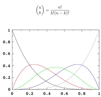
The Bernstein Polynomials of degreenare defined by:

B_kⁿ(t) = n

k

t^k(1−t)^(n−k) k= 0, . . . , n , (15)

(13)

where n

k

is the binomial coefficient:

n k

= n!

k!(n−k)!. (16)

Figure 5: Bernstein polynomials of degree n=4

Proposition 3.1 Basis: the Bernstein polynomials of degree nform a basis of Pⁿ, vector space of the polynomials of degree smaller or equal ton.

Proposition 3.1 justifies the choice of chosing Bernstein polynomials as basis functions.

Proposition 3.2 Degree Elevation: letP(t)∈ Pⁿ be represented in the Bernstein polynomials basis of degreenby the vector of coefficients p∈Rⁿ⁺¹, hence the representation p˜of P(t)in the Bernstein polynomials basis of degreen+ 1is







˜

p0 = p0

˜

pk = _n+1^k pk−1+

1−_n+1^k

pk, 1≤k≤n

˜

pn+1 = pn

(17)

The degree elevation is the key property to the hierarchical method which will be introduced in section 5.4. This provides a method to express any polynomials of degreenin any polynomials spaces of higher degree in the Bernstein basis.

(14)

Proposition 3.3 Unity Partition:

∀n, Xn

k=0

Bⁿ_k(t) = 1, ∀t

Proposition 3.3 shows how to use theFFD method for a one dimension deformation and such that the deformation is constant in this dimension. For instance, let ~pkxkz =~pkx, for allkz. Hence, according to (14), the deformation reads

∆x

∆z

=

nx

X

kx=0

B_kⁿ_x^x(tx)~pkx

nz

X

kz=0

B_kⁿ_z^z(tz)

| {z }

=1

=

nx

X

kx=0

B_kⁿ_x^x(tx)~pkx. (18)

4 Inverse problem: optimizing the shape of a reflector

In the direct problem, the radiation diagram can be computed providing a geometry and a source. Inversely, considering the geometry as the unknown, how can be determined the shape ofS to fit a given target diagram ?

To solve this inverse problem a shape functional that penalizes the discrepancy with the given diagram is minimized. First, the shape functional is defined and then different strategies to reduce it are discussed.

4.1 Shape functional

LetE~^t be the target electric field known on the planesϕ= 0andϕ= ^π₂ (one reminds from section 2.3 that this is sufficient to deduce the far field everywhere else). J1(S) is defined as the L2-norm of the difference between the field given by the current shape S (moving during the optimization process) andE~^t:

J1(S) = 1 2

Z 2π 0

kE(S, θ)~ −E~^t(θ)k²C²dθ. (19)

4.2 Parametric functional

Considering the parametric representation ofS (11) with theFFD technique (14), given a degree of parameterization(nx, nz), the meridianCdefined by the so-called shape parameters

~

pkxkz becomes:

C(p) =C⁰+ ∆C(p) =C⁰+

nx

X

kx=0 nz

X

kz=0

B_kⁿ_x^x(tx)B_kⁿ_z^z(tz)~pkxkz, (20)

(15)

from whichS(p)is derived by axisymmetry. Thus a parametric functionalj(p)is defined as follows:

j(p) =J(S⁰+ ∆S(p)), (21)

whereJ is given by (19). Finally, the optimization problem reads then:

p∈minR2×dj(p), (22)

wheredstands for the dimension of the deformation spaceX. Note thatd= (nx+1)(nz+1) with the considered basis functions.

5 Numerical case study

As for several inverse problems, the existence of the solution nor its uniqueness, if there exists one, is ensured. Consequently, these problems are usually hard to solve numerically.

Therefore, in order to be able to investigate the problem, a test-case is built such that the existence of a solution is established. Namely, the target field will come from a known geometry. This kind of problem is called areconstruction problem.

Two different methods have been considered: a gradient-based, deterministic one, and a semi-stochastic one. Solve a numerical optimization problem implies the use of softwares.

So, for each method, an experimentation is performed to ensure that the software is valid.

Then a few tests on the problem itself are carried out.

5.1 Case settings

The initial shapeS⁰ of meridianC⁰is defined as follows:

C⁰

x0(t) =t

z0(t) =zc . (23)

The target diagram corresponds to the computed diagram ofS^t with meridianC^t: C^t

x(t) =t

z(t) =zc+P(t) , (24)

for someP(t)∈ P^m(see Figure 6). The difference between the two curves is non zero only in thezdirection and is polynomial:

∆x

∆z

= 0

P(t)

. (25)

If a FFD deformation of degree(n,0) is considered, in the z direction only, the corresponding deformation space is spanned by the family{B_kⁿ}ⁿ_k=0of dimensiond=n+1. Since

(16)

this family is a basis of Pⁿ (see proposition 3.1), then for all n ≥ m, ∆z belongs to the deformation space. In other words,

∀n≥m,∃p= (p0. . . pn)∈Rⁿ⁺¹ ; ∆z(t) = Xn

k=0

pkB_kⁿ(t), (26) wherepis unique for each fixednsince this is simply the representation ofP(t)in a basis.

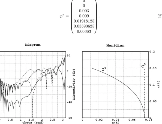
So, this test-case is well defined to validate our optimization routines: a solution exists and, by construction, this solution, noted p^∗, is known. This problem can be seen as a reconstruction problem more than a real optimization problem. In the concrete example in Figure 6 where∆z∈ P⁶(and is exactly of degree 6), forn=m= 6,p^∗ reads:

p^∗=





 0 0 0.003 0.009 0.01918125 0.03590625 0.06363







. (27)

0 0.5 1 1.5 2 2.5 3

theta (rad)

-60 -40 -20 0 20

Directivity (db)

Diagram

0 0.02 0.04 0.06 0.08

z(t)

0 0.05 0.1 0.15 0.2

x(t)

Meridian

C_t C⁰

Figure 6: initial and target diagrams (left) / shapes (right), ∆z∈ P⁶

Remark One can check that for allk > 0, Bⁿ_k(0) = 0and B₀ⁿ(0) = 1. Thus, in order to ensure condition (10),p0= 0. Actually, any point on the line x= 0will not be deformed.

(17)

This implies that with degree of parameterizationn, there arendegrees of freedom for each direction of deformation.

5.2 Gradient-based strategy

The Quasi-Newton methods are gradient-based optimization methods. They require the knowledge of the gradient while the Hessian is estimated through the iterations. This ensures quadratic convergence around the solution since the quadratic approximation of the functional becomes accurate.

5.2.1 Introduction to FFSQP

TheFFSQP[12] routine is a powerful Quasi-Newton implementation with BFGS update [11].

It is based on Sequential Quadratic Programming (SQP) and ensures all inequality and equality constraints. This routine has been chosen for its maturity.

5.2.2 Application to the case

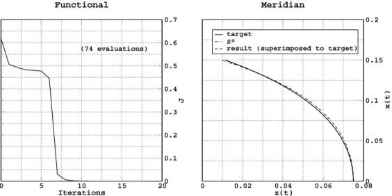
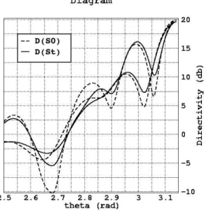
Method validation: First, consider a small perturbation of C^t as initial shape instead of C⁰ in Figure 6 and the highest degree, n = 6. Namely, C⁰ is deformed with parameter p= p^∗+δp for some non-zero δp ∈R⁷ (see Figure 8). Since the initial shape is close to the target one, close diagrams and consequently a fast converge are expected with such a method because the second-order Taylor expansion of the functional becomes accurate in the neighborhood of the solution. However note that such a perturbation in the shape has a non-negligible effect on the diagram: initialD(S⁰, θ)and targetD(S^t, θ)directivities are depicted in Figure 7. One focuses on the main directions θ∈ [2.5, π]where the difference mostly appears.

As expected, after fewer than 20 iterations the target diagram has been found (J(p)→0), as well as the target shape (both curves are superimposed, see Figure 8).

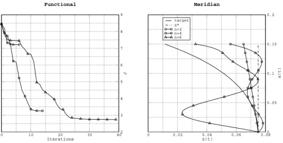
Case resolution: After the above validation, the considered case is solved for different degrees: n= 2,4, and6. Obviously, the target shape cannot be found whenn <6because in these cases∆z /∈X. One simply hopes to find a good approximation with fewer degrees of freedom.

It appears in Figure 9 that the shapes at convergence of the algorithm are very far from the target. The greater the degree, the closer is the diagram, however they are still very different (J(p)>2). Since a descent method is supposed to find the closest pointpfrom the initial value such thatJ⁰(p) = 0, one can suppose that the algorithm has converged towards some local minima.

Functional study: After the previous experimentations one may think that the functional is highly sensitive to shape perturbations and that there might be many local minima. In order to check these assumptions, let us evaluate the functional around the solution for some

(18)

Figure 7: initial and target diagrams

0 5 10 15 20

Iterations

0 0.1 0.2 0.3 0.4 0.5 0.6 0.7

J

Functional

0 0.02 0.04 0.06 0.08

z(t)

0 0.05 0.1 0.15 0.2

x(t)

target S°

result (superimposed to target) Meridian

(74 evaluations)

Figure 8: stability around the solution -FFSQP

(19)

0 10 20 30 40 Iterations

2 3 4 5 6 7 8 9

J

Functional

0 0.02 0.04 0.06 0.08

z(t)

0 0.05 0.1 0.15 0.2

x(t)

target S°

n=2 n=4 n=6

Meridian

Figure 9: numerical solutions w.r.t degree -FFSQP

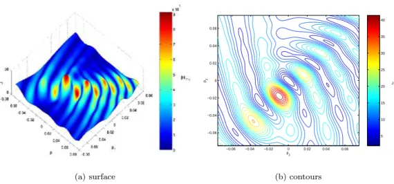
parameters. For a sake of simplicity a 2-parameters problem is considered. The target shape is the starting shape so that the solution yieldsp=~0. Then consider a FFD deformation for degreen= 2and set p0= 0as explained in the remark of section 5.1. Thus the functional is computed w.r.t. parametersp1 andp2as shown in Figure 10.

Clearly the functional has many local minima and hence the solution given by a descent method depends on the initial shape. In other words, if the initial shape is close enough to the target shape, that is, if it is in the neighborhood around the solution for which the functional is locally convex, then the algorithm will converge towards the target.

In addition the Froebenius-norm of the Hessian (evaluated by Finite Differences) is depicted in 10 with a color scale. One can see that the convex curvature is, for this norm, maximum at the minimum of the functional (see also Figure 11).

It has been shown in [6] that the wave length has a “dilatation” effect on the functional.

Namely, if the wave length is of the dimension of the antenna, then the functional looks unimodal for deformations that keep the shape in this dimension. This implies that one should measure the target field for one specific frequency or for multiple frequencies. In pure reconstruction problems, very good results for single and multiple frequencies can be seen in [6].

However, in optimization problems the target is the directivity, not the shape itself. In this case the scattered field at lower frequencies is unknown. Hence the “dilatation effect”

of the functional cannot be used since the considered frequency cannot be changed. It was shown previously that the functional is highly multimodal w.r.t. the chosen shape parameters.

(20)

(a) surface

5 10 15 20 25 30 35 40

−0.06 −0.04 −0.02 0 0.02 0.04 0.06

−0.06

−0.04

−0.02 0 0.02 0.04 0.06

p₁ p2

J

(b) contours

Figure 10: representation of the functional around the solution w.r.t. FFD shape parameters p1 andp2: degreen= 2,p0= 0,S⁰=S^t, solutionp= (0 0 0)^T

−0.08 −0.06 −0.04 −0.02 0 0.02 0.04 0.06 0.08

−40

−30

−20

−10 0 10 20 30

J dJ/dp₁⋅ 10⁻² d²J/dp₁²⋅ 10⁻⁴

Figure 11: functional, first and second derivatives w.r.t. p1 withp2= 0

(21)

Two configurations can be considered. if one has a good estimation of an initial shape, which can be the case for practical engineering problems, this method can be performant.

An example is given in Figure 12 where the initial shape is relatively close to the target one.

This configuration has been solved with degreenx= 15, nz= 1. S⁰ is a deformation of the same degree.

0 20 40 60 80

Iterations

1e-15 1e-10 1e-05 1

J

Functional

0 0.02 0.04 0.06 0.08

z(t)

0 0.05 0.1 0.15 0.2

x(t)

target S°

solution (superimposed to target) Meridian

Figure 12: reconstruction of a deformed antenna

Else, if one has no a priori knowledge about a good initial shape or wants to check the robustness of its initial guess, evolutionary algorithms may be more suitable.

5.3 Semi-stochastic strategy: Particle Swarm Optimization

TheParticle Swarm Optimization(PSO) method is an algorithm that was first developed to simulate bird flocks or fish schools. It has then been introduced as an optimizer [13]. Nowa- days there exits several improved versions but the main characteristics are well described in [14].

5.3.1 Introduction to the algorithm

ThePSO algorithm is a semi-stochastic, population-based, algorithm. The stochastic part comes from the use of random numbers to introduce diversity in the population. In so doing one hopes to avoid local minima through a global search. In the meanwhile some best solutions (to be defined) are kept in memory in order to influence the particles to search towards some directions.

(22)

Consider a classical unconstrained optimization problem inRⁿ:

p∈RminⁿJ(p) (28)

for some continuous objective functionJ. The key idea is to generate a sequence of popu- lations where at each iteration, each particle in the swarm moves in the search space with a certain velocity. The way the velocity is defined contains all the characteristics of the algorithm. Namely, it involves:

• the previous velocity (inertia);

• the swarm best solution (global trust);

• the personal best solution for each particle (self trust);

• a random effect.

Formally, the algorithm is described in Algorithm 1 and the algorithm variables are defined in Table 1.

Table 1: variable definition for PSO

P_i={p^j_i}^N_j=1 population at iterationi

V_i={v_i^j}^N_j=1 velocity vectors of the population at iterationi p^∗= Argmin_p∈{p^∗

0,...,p^∗_i}J(p) best particle so far (global trust) p^j∗= Argmin_p∈{p^j

0,...,p^j_i}J(p) best position found by particlej so far (self trust)

wi inertia coefficient at iterationi

wc inertia reduction coefficient

c1 self trust coefficient

c2 global trust coefficient

r1,r2 random numbers

Note that there are a few parameters to determine. Once they are fixed and once the random numbers sequences are generated, the evolution of the swarm is determined. The retained solution after the last iteration isp^∗. Since it is hard to define a convergence crite- rion, the number of iterations is usually fixed. However, there is a mechanical convergence when the inertia is reduced (wc < 1). In practice, there is no need to iterate when the inertia becomes smaller than a certain value. There is no diversity enough to look for other solutions. Therefore, if the standard deviation of the functional is smaller than a given value before iterationimax, the algorithm stops.

(23)

Algorithm 1Particle Swarm Optimization

Require: N,c1,c2,w0,wc,imax,p0,C⁰,(parameters to be determined) (1) First geometry : p0, C⁰

ComputeJ(p0) p^∗←p0

(2) Initialize uniformly the population and velocities in some subsetsD, D⁰⊂Rⁿ

(3) Loop

fori←0toimaxdo computeJ(p),p∈P_i updatep^∗,{p^j∗}^N_j=1

set random numbersr1and r2

V_i+1: v^j_i+1← wiv_i^j

| {z }

inertia

+c1r1(p^j∗−p^j_i)

| {z }

self trust

+c2r2(p^∗−p^j_i)

| {z }

global trust

P_i+1 : p^j_i+1←p^j_i+v_i+1^j

wi+1 ←wiwc {inertia reduction}

if std(J) <then quit loop end if

end for return p^∗

(24)

5.3.2 Application to the case

As in section 5.2, the stability of the algorithm around the solution is tested. Then the results for different degrees of parameterization are compared. In order to compare solutions for the same amount of computational work, the number of particles for each degrees is fixed to the valueN = 70. Moreover, the following parameters are set for all experimentations:

Parameter Value

w0 1.2

α 0.99

c1 2

c2 2

10⁻²

Method validation: Figure 13 shows that the algorithm is able to find the shape parameters that give the target diagram (J →0). However, compared to the descent method, the number of functional evaluations is much larger: 700011.

The algorithm is built so that there is a more global search at the beginning (with a large inertia) and a more local search at the end around the best solution found so far by the swarm. Since the first evaluation is close to the solution, one has to wait until the inertia becomes small enough so that p^∗ has enough influence on the swarm. Therefore, in this validation case, the number of evaluation is very large and there is not much improvement during the first iterations, i.e., during the global search. This can be seen in Figure 14.

Clearly, the swarm begins to converge around iteration 40: the functional mean begins to decrease and a better particle is found almost at each step (see Figure 13).

Case resolution: Now the case is solved for the same degrees as that used in section 5.2:

n= 2,4, and6. One can see in Figure 15 the results in terms of shape and functional.

With degree n = 2 one can see that the algorithm converges towards a shape that approximates quite well the target. As noted previously, with this degree the target is not reachable. Therefore the functional converges towards some non-zero value. Note also that the numerical solution is obtained after 50 iterations (3500 functional evaluations).

With n= 4the result is even better. The shape is actually almost superimposed to the target (it appears here that the chosen deformation∆zis almost of degree 4, but compared to the validation case, the value ofJ at convergence is still greater). However the algorithm is slower to converge: 100 iterations are needed to reach the best value (7000 functional evaluations).

At last, with n = 6one can see that 150 iterations are not sufficient to converge. The functional is still decreasing but far from 0.

More generally, the greater the degree, the slower the algorithm converges. It is quite intuitive that it is more difficult to explore a much larger domain with fewer particles. In [11]

this phenomenon is called the “curse of dimensionality”.

(25)

0 20 40 60 80 100 Iterations

0 0,1 0,2 0,3 0,4 0,5 0,6

J

7000 evaluations Functional

0 0,02 0,04 0,06 0,08

z(t)

0 0,05 0,1 0,15 0,2

x(t)

target S°

result (superimposed to target) Meridian

Figure 13: stability around the solution

0 20 40 60 80 100

iterations 0

10 20 30 40

J

particle mean best functional

Swarm functional

nparticules=70, n=6

Figure 14: swarm functional values ; when no better solution has been found at another point of the search space (significantly far), the whole swarm is attracted by the best particle, thus the functional mean value converges towards the best value (here the convergence begins around the 50th iteration).

(26)

0 50 100 150 200 Iterations

0 1 2 3 4

J

Functional

0 0.05 0.1

z(t)

0 0.05 0.1 0.15 0.2

x(t)

target S°

n=2

n=4 (superimposed) n=6

Meridian

Figure 15: numerical solutions w.r.t. degree,PSO

In the following section a strategy is proposed to obtain a solution with the highest accuracy (with n = 6) for at most the same amount of computational work (at most 150 iterations with 70 particles).

5.4 Towards a multilevel method with PSO

Hierarchical approaches for shape optimization with Bézier parameterization and inspired by the multi-grid theory has been recently introduced and applied in aerodynamic design [8, 9].

From simple level increase to Full Multi-Grid, this strategy is based on embedded parameterizations of increasing degree. This previous methods have been used with a gradient-based and a simplex optimizers. Here, a semi-stochastic multilevel algorithm is considered. The simple case, with only degree elevation, is considered.

5.4.1 Multilevel PSO

Starting from a parameterization of degree n = 2the best shape parameters noted p^∗2 is kept in memory. According to proposition 3.2 the same deformation can be expressed in the basis of degreen= 4by 2 successive degree elevations. The correponding shape parameters is noted p^∗4. Hence one can use p^∗4 as first best solution for another few iterations of PSO. In addition, since one has now an approximation of the solution from the coarse parameterization, the initialization domain is reduced around it and the inertia value is kept. More precisely, letB∞(p^∗, ρ)≡ {p∈Rⁿ;||p−p^∗||∞≤ρ}. Thus the first initialization domain is defined asD0=B(p0, ρ0)for someρ0>0and thenρis reduced at each elevation.

(27)

And so on for all considered degrees. The new algorithm reads in Algorithm 2. This strategy intends to avoid the issues due to the large dimensionality on the finer parameterization.

Algorithm 2Multilevel Particle Swarm Optimization

Require: N,c1,c2,w0,wc,imax,p0,C⁰,ρ0,β (parameters to be determined) Require: ki,i= 1. . . n: degree of parameterization for leveli,k1< k2<· · ·< kn

(1) First geometry : p0 inR^k¹,C⁰ ComputeJ(p0)

p^∗k¹←p0

D0←B∞(p0, ρ0) (2) Loop over degrees fori←1ton−1do

imaxiterations ofPSO updatep^∗kⁱ

p^∗kⁱ⁺¹←elevation(p^∗kⁱ) ρi+1←βρi

Di+1←B∞(p^∗kⁱ⁺¹, ρi+1) end for

(3) Finest degree imaxiterations ofPSO updatep^∗kⁿ

p^∗←p^∗kⁿ return p^∗

5.4.2 Application to the case The following parameters are used:

Parameter Value

w0 1.2

α 0.99

c1 2

c2 2

ρ0 0.150

β 0.20

In addition, let imax = 40 for the first two levels and imax = 70 for the last one. In Figure 16 the results obtained with the multilevel algorithm and the single parameterization PSO are compared. It is important to reduce the initialization domain on the finer grids.

(28)

If not, one would not make use of the information of the best solution from the previous parameterization.

0 50 100 150 200

Iterations

0 2 4

J

n=2 n=4 n=6 n=2->4->6

Functional

80 90 100 110 120 130 0 1e-06 2e-06 3e-06 4e-06 5e-06

Figure 16: comparison of the functional evolution for singelPSO with multilevelPSO with progressive degree elevation2→4→6

(29)

6 Conclusion

A conformation of axisymmetric antennas problem has been considered. The functional reads as the L2-norm of the difference between a measured field (or target field) and the computed field, given a geometry of reflector. AFree-Form Deformation method has been adopted to represent parametrically the deformation of an initial shape. The optimization problem consists in finding the minimal value of the functional (in particular, 0 for a reconstruction problem).

With such a configuration it has been shown that the problem is usually hard to solve since the functional is highly multimodal, even with 2 degrees of freedom. Thus, when there is no a priori knowlegde about the initial shape, a deterministic method has no chance to converge towards a global solution. However, when a better initial shape is given, the diagram can be significantly improved.

Then a semi-stochastic method, the Particle Swarm Optimization method, has been discussed. First, as expected, it appears that such a method is more robust since it is no more sensitive to local minima. However, this method requires more evaluations of the functional. When the degrees of freedom number increase, the problem becomes almost unsolvable. Hence, only solutions with small degrees of freedom, and thus unaccurate, can be obtained.

At last a multilevel Particule Swarm Optimization algorithm, inspired from multilevel optimization methods used in aerodynamics, has been proposed. This latter algorithm appears to be the best method for such problems since it is both robust and accurate.

(30)

References

[1] P. F. Combes,Micro-Ondes, Dunod (1997) vol. 2 chapters 5, 11.2, 12.3.1, 13.4.2 [2] R. Bills,Problème extérieur pour les equations de Maxwell Application aux antennes

de révolution, Thèse de doctorat, Université de Nice (1982)

[3] S. J. Orfanidis, Electromagnetic Waves and Antennas, Rutgers University (2004), http://www.ece.rutgers.edu/~orfanidi/ewa

[4] Wikipédia,Antenne — Wikipédia, l’encyclopédie libre, (2006),

http://fr.wikipedia.org/w/index.php?title=Antenne&oldid=7941063

[5] M. Leveque, Conformation et optimisation des antennes à réflecteur, stage réalisé à France Télécom R&D La Turbie (2000)

[6] P. Dubois, Optimisation de structures rayonnantes métalliques 3D par déformation de surfaces iso-niveaux en régime harmonique, Thèse de doctorat, École des mines de Paris (2005)

[7] T. Sederberg and S. Parry, Free-Form Deformation of Solid Geometric Models, Computer Graphics (1986)

[8] J.-A. Désidéri, B. Abou El Majd, A. Janka, Nested and Self-Adaptive Bézier Parameterizations for Shape Optimization, International Conference on Control, Partial Differential Equations and Scientific Computing, Beijing, Science Press (Sept. 13-16, 2004)

[9] J.-A. Désidéri,Two-level Ideal Algorithm for Parametric Shape Optimization, Journal of Numerical Mathematics (2006)

[10] J. Picard,Paramétrisation hiérarchique pour l’optimisation d’un réflecteur, stage réal- isé à l’INRIA Sophia Antipolis (2004)

[11] P. E. Gill, W. Murray, M. H. Wright, Practical Optimization, Academic Press (1986)

[12] J. L. Zhou, A. L. Tits, C. T. Lawrence, User’s Guide for FFSQP Version 3.7:

a Fortran Code for Solvings Constrained Nonlinear (Minimax) Optimization Problems, Generating Iterates Satisfying All Inequality and Linear Constraints, Institute for Sys- tems Research, University of Maryland, College Park, MD 20742 (April 1997)

[13] J. Kennedy, R. Eberhart, Particle Swarm Optimization, IEEE International Con- ference on Neural Networks, Vol.4 pp.1942-1948 (Nov./Dec. 1995)

[14] G. Venter, J. Sobieszczanski-Sobieski,Particle Swarm Optimization, AIAA Jour- nal, Vol.41 No.8 (August 2003)

(31)

Unité de recherche INRIA Futurs : Parc Club Orsay Université - ZAC des Vignes 4, rue Jacques Monod - 91893 ORSAY Cedex (France)

Unité de recherche INRIA Lorraine : LORIA, Technopôle de Nancy-Brabois - Campus scientifique 615, rue du Jardin Botanique - BP 101 - 54602 Villers-lès-Nancy Cedex (France)

Unité de recherche INRIA Rennes : IRISA, Campus universitaire de Beaulieu - 35042 Rennes Cedex (France) Unité de recherche INRIA Rhône-Alpes : 655, avenue de l’Europe - 38334 Montbonnot Saint-Ismier (France) Unité de recherche INRIA Rocquencourt : Domaine de Voluceau - Rocquencourt - BP 105 - 78153 Le Chesnay Cedex (France)