This consists of a root conversion (Gathen and Gerhard, 1999, Algorithm 9.14), followed by a modulo reduction of the coefficients. The first is a compression, performed by arithmetic operations, which reduces the size of the polynomial entries. However, in all three applications, we show that these compression techniques represent a speedup factor typically of the order of the number k of residues stored in the compressed format.
Here we give an improved version of concurrent reduction where the number of operations is divided by two. We also give a complete study of the behavior of integer division by floating-point subroutines, depending on the rounding methods. In Section 6 we show that it is also possible to tabulate the evaluations at q and that we can directly access the required part of the machine words (using e.g. bitfields and unions in C) instead of performing a radix conversion.
The first improvement we propose to the DQT is to replace the costly modular reduction of the polynomial coefficients (for example, in step 4 of algorithm 1) with a single division by p followed by several shifts. This proves that the operations can be performed independently on the different parts of the machine words. When q is a power of 2, the calculation of the ui in the first part of algorithm 2 requires 1 div and (k+ 1)/2 axpy as shown in Theorem 8.
The inverse of the prime number can be pre-computed for each mode, changing costly modes.
Rounding Modes
Floating Point Division
Results
If it is a power of 2, then the way to round k(1−2−β) is the same as for 1−2−β, since it only changes the exponent in the result.
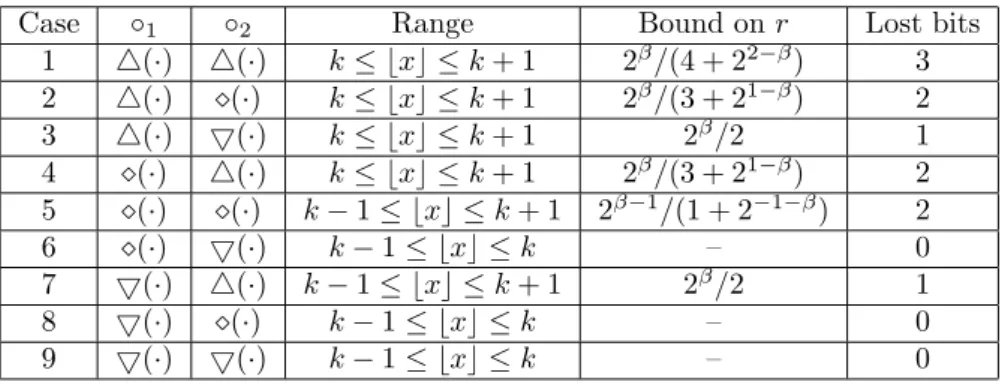
Bounds on r making the result exact
The limit on r follows from case 3, since ǫ1 and ǫ2 play a symmetric role in the error analysis of case 3.
Using Algorithm 4
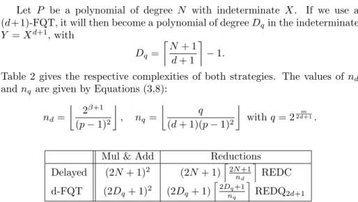
Delayed Reduction
Fast Q-adic Transform
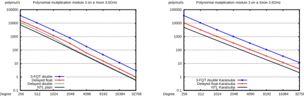
Comparison
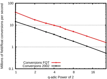
If we choose a double floating point representation and a 4-FQT (ie 4 coefficients in a word, or a power 3 substitution), the fully tabulated FQT boils down to 8.6·104 multiplications and additions and 5.7· 103 divisions. Even by switching to a larger mantissa, e.g. 128 bits, so the DQT multiplications are about 4 times as expensive as double floating point operations, the FQT can still be useful. We see that FQT is faster than NTL as long as the same algorithm is used.
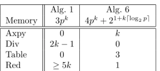
Moreover, it is possible to use floating point routines to perform exact linear algebra, as shown by Dumas et al. We use the strategy of (Dumas et al., 2002, Algorithm 4.1): convert vectors over Fpk to q-adic floating point; call a fast numerical linear algebra routine (BLAS); convert the floating point result back to the usual field representation. Algorithm 6Fast Dot Product over Galois Fields via FQT and FQT Inverse Input: A field Fpk with elements represented as exponents of a generator of the .
Thus, this algorithm approaches the performance of fringe wrapping even for small extension fields. Suppose that the internal representation of the expansion field is already with discrete logarithms and uses conversion tables from polynomial to index representations (see e.g. Dumas (2004) for details). We then choose a tradeoff between time and memory for a REDQ operation of the same order of magnitude, that is, saypk.
This reduction can be pre-calculated when looking up the REDQ table and is therefore almost free. For example, elements are represented by their discrete logarithm with respect to the field generator instead of polynomials. Here, q is a power of two and division REDQ is calculated using the floating-point routines of Section 4.
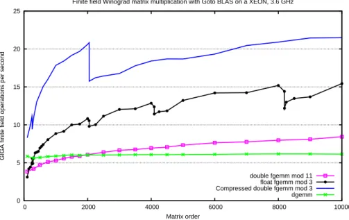
This represents a reduction from the 15% overhead of the previous implementation to less than 4% now, compared over F11. 4On a XEON, 3.6 GHz, using Goto BLAS-1.09dgemms the numerical routine (Goto and van de Geijn, 2002) and FFLASfgemm for the fast prime field matrix multiplication (Dumas et al., 2009). 5The FFLAS routines are available within the LinBox 1.1.4 library (LinBox Group, 2007) and the FQT is implemented in thegivgfqext.hfile of the Givaro 3.2.9 library (Dumas et al., 2007).
Middle Product Algorithm
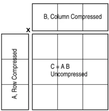
We investigate the possibilities of left-only or right-packing along with packing on both matrices of a matrix multiplication. In terms of the number of arithmetic operations, the matrix multiplication CA×CB can save a factor ofd+ 1 over the multiplication of A×B as shown in the 2×2 case above. The compression and extraction are less demanding in terms of asymptotic complexity, but can still be noticeable for moderate sizes.
This is done in Section 7.6 (Table 5), where the actual matrix multiplication algorithm is also considered. Note that the last column of CA and the last row of B may not have + 1 elements if d+ 1 does not divide k.
Available Mantissa and Upper Bound on Q for the Middle Product
Middle Product Performance
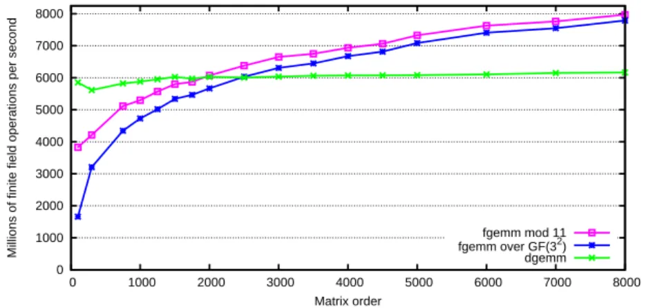
Geijn (2002) and for the fgemmmodular matrix multiplication of the FFLAS-LinBox library by Dumas et al. This figure shows that the (d+ 1) compression is very efficient for small primes: the gain over the double floating-point routine is quite close. In fact, the matrix starts to be too large and modular reductions are now required between the recursive matrix multiplication steps.
Then BLAS floating-point routines are used only when the sub-matrices are small enough. In Table 4, we show compression factors modulo 3, with a Qa power of 2 to speed up conversions. Then from dimensions 257 to 2048 one has a factor of 4 and the times are approximately 16 times the time of the four times smaller matrix.
It would be interesting to compare the multiplication of 3-compressed matrices of size 2049 with the decomposition of the same matrix on matrices of size 1024 and 1025, thus allowing 4-compression even for matrices larger than 2048, but with more modular reductions.
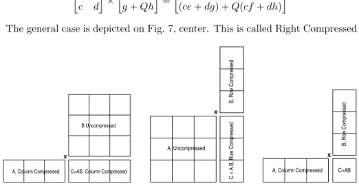
Right or Left Compressed Matrix Multiplication
We see in Figure 8 that using REDQ instead of the middle product algorithm has a major advantage. Indeed, for small matrices, the conversion can represent 30% of the time and any improvement there has a big impact.
Full Compression
CMM Comparisons
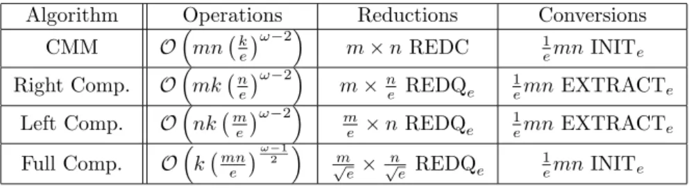
For small matrices, the conversion can actually represent 30% of the time, and any improvement there has a big impact. where, as above, β is the magnitude of the mantissa and Q is the integer chosen according to Eq. 9) and (10), except for full compression, where the more limited Eq. Thus, the degree of compression for the first three algorithms is justd=e−1, while it becomes onlyd=√. In terms of asymptotic complexity, the cost in number of arithmetic operations is dominated by that of the product (column Operations in the table), while reductions and conversions are linear in dimensions.
For example, with the algorithm Right compression on matrices of sizes, it took 90.73 seconds to execute the matrix multiplication module 3 and 1.63 seconds to convert the resulting matrix. There, conversions account for 43% of the time, and it is therefore extremely important to optimize conversions. In the case of rectangular matrices, the second column of Table 5 shows that one should choose the algorithm depending on the largest dimension: CMM if the common dimension is the largest, Right compression if the largest and Left compression if mdominates.
The gain in terms of arithmetic operations is eω−2 for the first three variants and eω−21 for full compression. The full compression algorithm appears to be the best candidate for locality and use of fast matrix multiplication; however, the compression factor is an integer, depending on the floor covering of both logβ. There are thus matrix dimensions for which the compression factor for e.g. the real compression will be greater than the square of the compression factor of the full compression.
If the matrices are squared (m = n = k) or if ω = 3, the products all become the same, with similar constants implied in theO(), so that locality considerations aside, the difference between them is the time spent in discounts and conversions. Since REDQ reduction is faster than classical reductions (Dumas, 2008), and since INITe and EXTRACTe are roughly the same operations, the best algorithm would be one of left, right, or full compression. Further work includes implementing the full compression and comparing the actual timing of the conversion overhead with that of the Right algorithm and that of CMM.
It turns out to be efficient for modular polynomial multiplication, expansion fields conversion to floating point, and linear algebra routines over small prime fields. It will also be interesting to see in practice how this trick extends to higher precision implementations: on the one hand the basic arithmetic slows down, but on the other hand the trick enables a more compact packing of elements (e.g. if an odd number of field elements can be stored within two machine words, etc.). Eds.), Proceedings of the Seventh International Workshop on Computer Algebra in Scientific Computing, Yalta, Ukraine.