It will therefore be stated that the flow curvature method, which uses neither eigenvectors nor asymptotic expansions, but only involves time derivatives of the velocity vector field, is a general method that simplifies and improves the slow invariant manifold analytical equation determination of high. -dimensional dynamical systems. Curvature4 measures, so to speak, the deviation of the curve from a straight line in the vicinity of any of its points. The main result of this work presented in the first section establishes that curvature of the flow, i.e. curvature of trajectory curves of any n-dimensional dynamical system, directly provides its slow multiple analytic equation whose invariance is proved by Darboux theorem.
Thus, the approximation method of the tangent linear system provided the slow multiple analytic comparison of low-dimensional dynamical systems according to the "slow" eigenvectors of the tangent linear system, i.e. according to the "slow" eigenvalues. Also to solve this problem it was necessary to make such an equation independent of the "slow" eigenvalues. Thus, the main result of this work established in the next section is that the curvature of the flow, i.e. the curvature of trajectory curves of any n-dimensional dynamical system directly yields its slow multiple analytic equation whose invariance is determined by the theorem from Darboux.
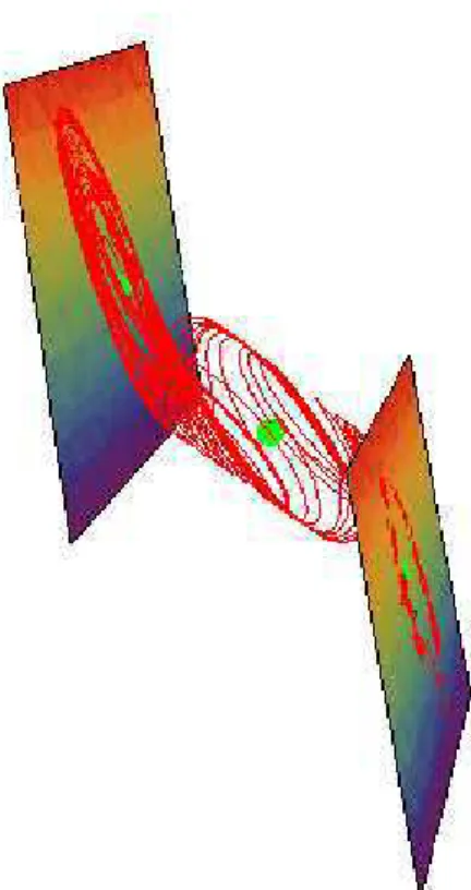
Since it uses neither eigenvectors nor asymptotic expansions, but simply includes the time derivatives of the velocity vector field, it represents a general method that simplifies and improves the determination of the slow invariant analytical equation of the manifold of high-dimensional dynamical systems. In what follows, the invariance of the slow manifold will be established according to what will be called Darboux's theorem. The curvature of the current indicates that the location of the points where the second curvature (torsion) of the current, ie. the second curvature integral of the path curves of the Chua system, vanishes, directly provides its slow invariant analytic manifold equation, i.e. equations of planes (Π).
Moreover, since Chua's system (10) is piecewise linear, the time derivative of the functional Jacobian matrix is zero: djdt = 0.
Four-dimensional Chua’s system
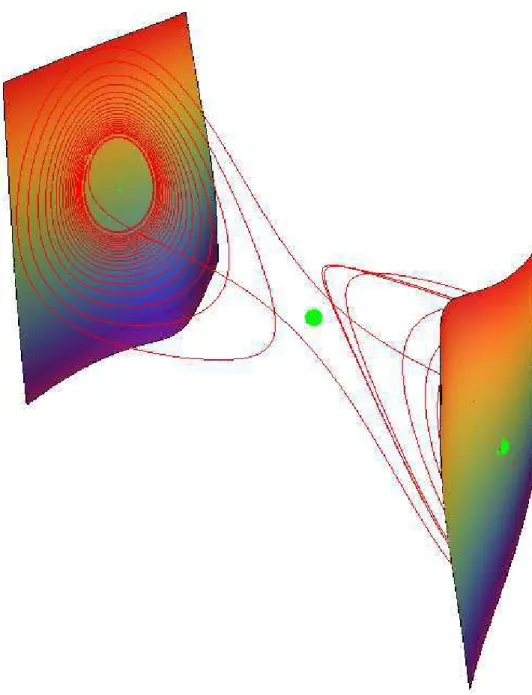
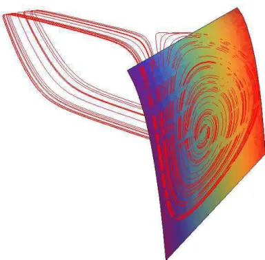
The flow curvature states that the locus of the points where the third flow curvature, i.e., the third curvature of the integral trajectory curve of Chua's fourth-order system, vanishes directly provides its slow invariant analytical equation , i.e. Π) equations of hyperplanes. 0 Then, prove that the (Π)hyperplane equation (23) is factorable in Eq. 24) and so both methods provide the same equations of hyperplanes. Furthermore, in the framework of Differential Geometry, the hyperplane (Π) can be interpreted as theoscillating hyperplane passing through every fixed point I1 (respectively I2).

Five-dimensional Chua’s system
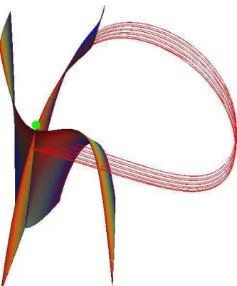
The curvature of the current states that the location of the points where the fourth curvature of the current disappears, ie. (Π)equations of hyperplanes. The partially linear characteristic and the two identities (59) and (61) make it possible to state, in accordance with Darboux's theorem [1878], that the polyhedra is φ. 33) is exactly the same as Eq. 0 He then proves that the equation of the (Π)hyperplane (31) is a factor in Eq. 32) and so that both methods provide the same hyperplane equations.
After these tutorial examples regarding Chua's piecewise linear systems, let's apply the curvature of the flowton linear Chua's cubic systems of dimension three, four and five.

Three-dimensional cubic Chua’s system
Four-dimensional cubic Chua’s system
Five-dimensional models
The first is a fifth order nonlinear model of magnetoconvection [Knobloch et al., 1981], for which a slow invariant manifold will be provided directly using flow curvature. The latter is a fifth-order artificial nonlinear model [Gearet al., 2005], which has three attractive invariant manifolds.

Five-dimensional magnetoconvection model
Five-dimensional nonlinear model
During the twentieth century, various methods have been developed to determine the slow invariant manifold analytic equation associated with slow-fast dynamical systems or singularly perturbed systems, among them the so-called Geometric Singular Perturbation Theory [Fenichel 1979] and the Tangent Linear System Approximation [Rossetto et al. 21] the problem of finding the slow in-variant manifold analytic equation with Geometric Singular Perturbation Theory turned into a regular perturbation problem where one generally expected the asymptotic validity of such an expansion to collapse. Moreover, slow invariant manifold analytical equation determination leads to tedious calculations for high-dimensional singly perturbed systems.
The approximation of the Tangent Linear System, the generalization of which is presented in the appendix, has given the slow manifold-analytic equation of non-dimensional dynamical systems according to the "slow" eigenvectors of the tangent linear system, i.e., according to the "slow" eigenvectors. Furthermore, starting from the dimension FiveGalois Theory excludes from the analytical calculation of the eigenvalues associated with the functional Jacobian matrix of a five-dimensional dynamical system. In this paper, considering the trajectory curves, integrals of n-dimensional dynamical systems, in the framework of Differential Geometry as curves in n-Euclidean space, it is proved that the curvature of the flow, i.e., the curvature of the trajectory curves of any dynamical system n-dimensional directly provides its slow multiple analytic equation, whose invariance is proved according to the Darboux theorem.
It is therefore stated that since curvature only involves time derivatives of the velocity vector field and does not use eigenvectors or asymptotic expansions, this simplification method improves the slow invariant multiple analytical equation determination of high-dimensional dynamical systems. Since it was shown in the appendix that curvature of the flow generalizes the Tangent Linear System Approach and includes the so-called Geometric Singular Perturbation Theory, it can be applied for slow invariant manifold determination of various types of high-dimensional dynamical systems such as Chemical kinetics, Neuron Bursting models, L.A.S.E.R. It seems reasonable to consider that a bifurcation will change the shape of the manifold and, conversely, geometrical interpretations may make it possible to highlight such bifurcations.
2004] "Projection on a slow manifold: singularly perturbed systems and legacy codes", SIAM Journal on Applied Dynamical Systems, preprint. The purpose of this appendix is to present definitions inherent to Differential Geometry such as the concept of non-dimensional smooth curves, the generalized Frénet frame, the Gram-Schmidt orthogonalization process for calculating the curvatures of trajectory curves in Euclidean space, as well as evidence A.10, A.15. & A.16) used in this work. Then, it is found that the flow curve for the slow determination of the multiple invariant analytical equation of high-dimensional dynamical systems generalizes on the one hand the tangent linear system approximation [Rossetto et al., 1998] and on the other hand thus includes -e called Geometric Singular Perturbation Theory [Fenichel, 1979].
Within the framework of Differential Geometry, n-dimensional smooth curves, i.e. smooth curves in Euclidean n-space, are defined by a regular parametric representation in terms of arc length, also called natural representation or unit speed parametrization. According to Herman Gluck [1966], local metric properties of curvatures can be derived directly from curves parametrized in terms of time and no sonatural representation is necessary.
Concept of curves
Gram-Schmidt process and Frénet moving frame
These vectors~ui(t) can be determined by applying the Gram-Schmidt orthogonalization process described below.
Frénet trihedron and curvatures of space curves
Identities proofs
Assumptions
Corollaries
Yλi (69) Then, the existence of an evanescent mode in the slow multiple vicinity implies according to Tikhonov's theorem [1952] thata1λ1 ≪1. The coplanarity condition between the velocity vector field−→ V of an n-dimensional dynamical system and the slow eigenvectors. The star λi associated with the slow eigenvalues of its functional jacobian provides the slow multiple equation of such a system.
1998] uses the "fast" eigenvector on the left associated with the "fast" eigenvalue of the transposed functional Jacobian of the tangent linear system. V of an n-dimensional dynamical system and the fast eigenvector t−→. Yλ1 on the left, associated with the fast eigenvalue λ1 of its transposed functional Jacobian, provides the equation of the slow manifold of such a system. Since for low-dimensional two- and three-dimensional systems the proof was already established [Ginouxet al., 2006] using the tangent linear system approximation, for high-dimensional dynamical systems it can be derived from its generalization presented above.
Thus, according to the generalization of the Tangent Linear System Approximation, the slow manifold equation of a one-dimensional dynamical system can be written: Under the assumptions of the Tangent Linear System Approach, it is clear that the vectors. The functions f~en~gare are assumed to be C∞ functions of ~x, ~z and εin U×I, where U is an open subset of Rm×Rn and I is an open interval containing ε= 0.
When ε≪1, that is, is a small positive number, the variable ~x is called fast variable, and ~z is called slow variable. The independent variable stateτ is referred to the fast and slow times, respectively, and (75) and (76) are called fast and slow system, respectively. These systems are equivalent when ε 6= 0, and they are labeled as singular perturbation problems when ε≪1, that is, is a small positive parameter.
The label singular derives in part from the discontinuous limiting behavior of system (75) as ε → 0+. In such a case, system (75) reduces to an m-dimensional system called reduced fast system, where the variable is a constant parameter. System (76) leads to a differential-algebraic system called reduced slow system whose dimension decreases from m+nton. By exploiting the decomposition into fast and slowly reduced systems, the geometric approach reduced the fully perturbed system to separate lower-dimensional regular perturbation problems into fast and slow regimes, respectively.
Assumptions
Theorems