HAL Id: tel-00439782
https://tel.archives-ouvertes.fr/tel-00439782
Submitted on 8 Dec 2009
HAL is a multi-disciplinary open access archive for the deposit and dissemination of sci- entific research documents, whether they are pub- lished or not. The documents may come from teaching and research institutions in France or abroad, or from public or private research centers.
L’archive ouverte pluridisciplinaire HAL, est destinée au dépôt et à la diffusion de documents scientifiques de niveau recherche, publiés ou non, émanant des établissements d’enseignement et de recherche français ou étrangers, des laboratoires publics ou privés.
Discrete Complex Analysis
Christian Mercat
To cite this version:
Christian Mercat. Discrete Complex Analysis. Mathematics [math]. Université Montpellier II - Sciences et Techniques du Languedoc, 2009. �tel-00439782�
Habilitation ` a Diriger les Recherches en sciences
pr´esent´ee `a
l’Universit´ e de Montpellier 2
Sp´ecialit´e
Math´ ematiques
par
Christian Mercat
Sujet du m´emoire:
Analyse complexe discr`ete
pr´esent´ee et soutenue publiquement le mercredi 9 d´ecembre 2009 `a Montpellier devant le jury compos´e de
Pr. VladimirMatveev(universit´e de Bourgogne) Pr´esident du jury et rapporteur Pr. Jean-MarieMorvan(universit´e Claude Bernard, Lyon) Rapporteur
Pr. FrankNijhoff(universit´e de Leeds) Rapporteur Pr. Val´erieBerth´e(universit´e Montpellier 2) Examinatrice Pr. R´emy Malgouyres(universit´e d’Auvergne) Examinateur Pr. Jean-Pierre R´eveill`es(universit´e d’Auvergne) Examinateur
Curriculum Vitae 5
List of publications 7
Chapter 1. Presentation of scientific activity 9
1.1. Synthesis of work 9
1.1.1. Discrete Complex Analysis 9
1.1.2. Integrable Models 12
1.1.3. Exactly Solvable Models in Statistical Mechanics 15
1.1.4. Topology 16
1.2. PhD supervision 17
1.2.1. Diffusion processes 17
1.2.2. Discrete Laplacian 18
1.2.3. Digital Geometry 18
1.2.4. Fuzzy set 19
1.2.5. Discrete derivatives 21
Chapter 2. DiscreteRiemannSurfaces 23
2.1. Conformal maps 23
2.2. Real discrete conformal structure 28
2.2.1. Graphs and Discrete Conformal Structure 28
2.2.2. Complexes 29
2.2.3. Averaging forms 30
2.2.4. Hodgestar 31
2.2.5. Wedge product 31
2.2.6. Energies 32
2.2.7. Quasi-conformal maps 33
2.2.8. Abelian forms 34
2.2.9. Numerics with surfaces tiled by squares 35
2.2.10. Polyhedral surfaces 36
2.2.11. Towards a discreteRiemann-RochTheorem 38
2.3. Non real conformal structure 40
2.3.1. ComplexHodgestar 40
2.3.2. Surfel surfaces 41
Chapter 3. Discrete Complex Analysis and Integrability 45 3.1. Darboux-B¨acklundtransformation 46 3.2. Zero-curvature representation and isomonodromic solutions 47
3.3. Integrability and linear theory 48
3.3.1. Exponential 48
3
4 CONTENTS
3.3.2. Integration 50
3.3.3. Isomonodromic solutions, theGreenfunction 52
Chapter 4. Statistical Mechanics 55
4.1. The criticalIsingmodel 55
4.1.1. Boltzmannlaw 55
4.1.2. The fermionψ 56
4.2. The criticalA-D-E models 57
4.2.1. A-D-E models 57
4.2.2. Graph fusion algebra 59
4.2.3. Ocneanualgebra 60
4.2.4. CriticalA-D-E models 61
4.2.5. Fusion Projector 63
4.2.6. Fused face operators 64
Bibliography 67
Christian Mercat mercat@math.univ-montp2.fr I3M UMR 5149 Universit´e Montpellier 2 Phone: +33 4 67 14 42 33 Place Eug`ene Bataillon, c.c. 51 Fax: +33 4 67 14 35 58 F-Montpellier cedex 5 http://www.math.univ-montp2.fr/SPIP/_MERCAT-Christian_
Maˆıtre de conf´erence married, born July rd
Diplomas
PhD thesis at the Louis Pasteur University (Strasbourg), under supervision of DanielBennequin
Agr´egation de Math´ematiques
Magist`ere de l’´Ecole Normale Sup´erieure de Paris (M.Sc.)
Diplˆome d’´Etude Approfondie (Strasbourg)
- Ecole Normale Sup´erieure de Paris´ Professional Experience
Sept. - Maˆıtre de conf´erences (associate professor) at the Montpellier 2 University
- Postdoc at the Technical University Berlin
- Postdoc at the University of Melbourne
Sep.-Dec. Professeur agr´eg´e, Champlain highschool, Chennevi`ere/M.
Jan.-Aug. Postdoc at the Tel Aviv University, Israel
Sep.-Dec. Postdoc at theMittag-LefflerInstitute, Sweden Other Activities
- PhD supervision of Fr´ed´ericRieuxon digital diffusion and convolution applied to discrete analysis
- 3 M.Sc. in computer science supervisions.
- Member of the Directing Committee of the Pˆole MIPS (Mathematics, Computer Sc., Physics, Mechanics) of the University Montpellier 2
- Initiator of the Inter2Geo European project
- Partner of the Math-Bridge European project
Reviewer for SIGGRAPH, ACM Trans. On Graph., IWCIA, Duke Math. J., Adv. Appl. Math., J. of Math. Ph., Eur. Phy. J., J. Diff. Eq. Appl., L. in Math. Ph.; 15 reviews in MathSciNet.
Languages: French (native), English (fluent), German and Spanish (conversation) Computer: Java, C++, python, PHP, MySql, html, javascript, spip, joomla, xwiki,
mathematica, maple
[1] B Alexander Bobenko, Christian Mercat, and Markus Schmies. Conformal structures and period matrices of polyhedral surfaces. In A. Bobenko and Ch. Klein, editors, Riemann Surfaces - Computational Approaches, pages 1–13. 2009.
[2] C Ulrich Kortenkamp, Christian Dohrmann, Yves Kreis, Carole Dording, Paul Libbrecht, and Christian Mercat. Using the Intergeo Platform for Teaching and Research. The Ninth International Conference on Technology in Mathematics Teaching (ICTMT 9), Metz, France, July 6-9 (2009).
[3] V Applications conformes.Images des math´ematiques, Mar. 2009.http://images.math.
cnrs.fr/Applications-conformes.html.
[4] C Ulrich Kortenkamp, Axel M. Blessing, Christian Dohrmann, Yves Kreis, Paul Libbrecht, and Christian Mercat. Interoperable interactive geometry for europe - first technological and educational results and future challenges of the intergeo project. CERME 6 - Sixth Conference of European Research in Mathematics Education, Lyon, France, Jan. 28-Feb 1 (2009).
[5] V De beaux entrelacs.Images des math´ematiques, Feb. 2009.http://images.math.cnrs.
fr/De-beaux-entrelacs.html.
[6] C Discrete complex structure on surfel surfaces. Coeurjolly, David (ed.) et al., Discrete geometry for computer imagery. 14th IAPR international conference, DGCI 2008, Lyon, France, April 16–18, 2008. Proceedings. Berlin: Springer. Lecture Notes in Computer Science 4992, 153-164 (2008)., 2008.
[7] C Paul Libbrecht, Cyrille Desmoulins, Ch. M., Colette Laborde, Michael Dietrich, and Maxim Hendriks. Cross-curriculum search for Intergeo. Autexier, Serge (ed.) et al., Intelligent computer mathematics. 9th international conference, AISC 2008, 15th symposium, Calcule- mus 2008, 7th international conference, MKM 2008, Birmingham, UK, July 28–August 1, 2008. Proceedings. Berlin: Springer. Lecture Notes in Computer Science 5144. Lecture Notes in Artificial Intelligence, 520-535 (2008)., 2008.
[8] B Discrete riemann surfaces. In Athanase Papadopoulos, editor,Handbook of Teichm¨uller Theory, vol. I, volume 11 ofIRMA Lect. Math. Theor. Phys., pages 541–575. Eur. Math.
Soc., Z¨urich, 2007.
[9] V Keltische Flechtwerke.Spektrum der Wissenschaft, Special issue Ethnomathematik:46–
51, Nov. 2006.http://www.spektrum.de/artikel/856963.
[10] A Alexander I. Bobenko, Ch. M., and Yuri B. Suris. Linear and nonlinear theories of discrete analytic functions. Integrable structure and isomonodromic Green’s function.J. Reine Angew.
Math., 583:117–161, 2005.
[11] A Exponentials form a basis of discrete holomorphic functions on a compact.Bull. Soc.
Math. France, 132(2):305–326, 2004.
[12] A C. H. O. Chui, Ch. M., and Paul A. Pearce. Integrable and conformal twisted boundary conditions for sl(2)A-D-Elattice models.J. Phys. A, 36(11):2623–2662, 2003.
[13] B C. H. Otto Chui, Ch. M., and Paul A. Pearce. Integrable boundaries and universal TBA functional equations. In MathPhys odyssey, 2001, volume 23 of Prog. Math. Phys., pages 391–413. Birkh¨auser Boston, Boston, MA, 2002.
[14] A C. H. Otto Chui, Ch. M., William P. Orrick, and Paul A. Pearce. Integrable lattice realizations of conformal twisted boundary conditions.Phys. Lett. B, 517(3-4):429–435, 2001.
[15] A Ch. M. and Paul A. Pearce. Integrable and conformal boundary conditions for Zk
parafermions on a cylinder.J. Phys. A, 34(29):5751–5771, 2001.
7
8 LIST OF PUBLICATIONS
[16] A Discrete Riemann surfaces and the Ising model. Comm. Math. Phys., 218(1):177–216, 2001.
[17] T Holomorphie discr`ete et mod`ele d’Ising. PhD thesis, Universit´e Louis Pasteur, Strasbourg, France, 1998. under the direction of Daniel Bennequin, Pr´epublication de l’IRMA, available at http://www-irma.u-strasbg.fr/irma/publications/1998/98014.shtml.
[18] V Les entrelacs des enluminures celtes. Pour la Science, (Num´ero Sp´ecial Avril), 1997.
www.entrelacs.net.
[19] V Th´eorie des nœuds et enluminure celte. l’Ouvert, Num. 84:1–22, 1996, IREM de Strasbourg.
A Peer reviewed article B Peer reviewed book chapter C Peer reviewed conference proceeding T PhD Thesis
V Non peer reviewed vulgarization
Presentation of scientific activity
1.1. Synthesis of work
In this section, I will summarise my scientific work, going backwards in time, without going into too many details, the following chapters being more comprehen- sive.
My present interest is in Discrete Differential Geometry, especially applied to Computer Graphics, but it stems from Discrete Complex Analysis and Integrable Models, which has been my main subject of study during the past 6 years. The intention is to translate the best part of the theory of surfaces and complex analysis to the era of computers and discrete surfaces. This XIXth century theory, paved the way to the world of engineering marvels of the XXth century. Its discrete counterpart would be a real benefit for many different subjects of industrial interest.
I have developped the theory of Discrete Complex Analysis and DiscreteRie- mannSurfaces as a tool to tackle issues in Exactly Solvable Models in Statistical Mechanics. The main idea is to try to see, in an exactly solvable model, a Finite Conformal Field Theory, without having to go to the thermodynamic limit. This life long project, set by my advisor Daniel Bennequin, was given positive partial answers in my PhD thesis: criticality in the Ising model can be seen at the finite level as compatibility with discrete conformality.
1.1.1. Discrete Complex Analysis. This subject is at the heart of my work and most of my recent papers deal with it [6, 8, 10, 11]. The initial impulse, based on previous work by Lelong-Ferrand[62] and Duffin [59, 60], was given in my PhD thesis, summarized in Comm. in Math. Phys. [16, 17].
Analytic functions are everywhere, behind every key of hand-held calculators, like x 7→ x2, 1/x, tan, exp, log, and the theory of Riemann surfaces that gen- eralizes them on non flat surfaces has proven to be a highlight of XIXth century mathematics. Nowadays, Computer Graphics use it to globally parameterize dis- crete surfaces for a variety of reasons, texture mapping, segmentation, remeshing, animation...
At the root ofRiemannsurfaces is the concept of complex differentiability and line integration of complex valued functions. In order to discretize these notions, one needs a discrete version of exterior differential calculus, Hodge theory and Cauchy-Riemannequation.
Points in the Cartesian plane (x, y)∈R2gain in being seen as complex numbers x+i y ∈ C with the famous “imaginary” numberi such that i2 = −1. But the XVIth century trick, of manipulating the square root of negative numbers, is now as “real” as the real line of lengths, giving to the complex numbers the structure of a field, with addition and multiplication, unifying points of the plane and Euclidean transformations of them: ζ∈Cis whether a point, a vector acting by translation
9
10 1. PRESENTATION OF SCIENTIFIC ACTIVITY
when added, or a similitude when multiplied. The similitude z 7→ α z+β scales the whole plane by a factor|α|and turns it by an angle arg(α).
A holomorphic functionf is a complex differentiable function, that is a trans- formation of the plane which is, except at isolated critical points,locallya similitude and the local similitude factor is called thederivative f′ of the function:
f(z+z0) =f(z0) +f′(z0)×z+o(z).
At the zero of the derivative, the function behaves locally like a monomial z 7→
zk. Goursat noticed that simply asking for this local feature of differentiability
Figure 1.1: The pull-back of the picture of a clock paving the complex plane, by a polynomial (see Sec. 2.1). One can see the branchings at the zeros of the derivative where the zoom factor diverges.
actually implies that the derivativef′ is itself a holomorphic function. Compared to the vast zoo of differentiable real functions, complex differentiation is very rigid.
A natural discretization of these equations takes place on cellular decomposi- tions of surfaces byquadrilaterals of a given shape, the two dual diagonals locally playing the role of coordinates. With♦0, ♦1, ♦2 the vertices, edges and faces of a quad-decomposition, for each face (x, y, x′, y′) ∈ ♦2 (see Fig. 1.2), prescribe a certaindiagonal ratio ρon the unoriented edges:
ρ(x, x′) = 1
ρ(y, y′)=−iZ(y′)−Z(y) Z(x′)−Z(x)
for any realizationZ of the shape of the associated (oriented) quadrilateral in the complex plane. This ratio is by construction invariant by similitudes. It is real when diagonals are orthogonal (see Fig. 1.3). A functionf on the vertices is said to be discrete holomorphic if, for each such face, the diagonal ratio of the image is unchanged:
f(y′)−f(y) =iρ(x, x′) f(x′)−f(x) .
This equation is reminiscent of the Cauchy-Riemannequation when the diago- nals are orthogonal, mimicking local orthogonal coordinates and the compatibility between the partial derivatives.
x y
′x
′y
Figure 1.2: A quadrilateral (x, y, x′, y′) with a given shape in the complex plane.
ρ=12 ρρ= 1= 1 ρ= 2 ρ= 1 +i
Figure 1.3: Different quadrilateral shapes and the associated diagonal ratio.
Although very simple, this definition yields a lot of results similar to the con- tinuous theories of complex analysis andRiemann surfaces.
As in the continuous, there is a (infinitesimal) contour integration formula for the differentiation, analogous tof′(z0) = lim
γ→z0
i 2A(γ)
I
γ
f(z)d¯z:
f′(x, y, x′, y′) :=
I
∂(x,y,x′,y′)
f(z)d¯z,
but it is only in the case of flat rhombi decompositions that the derivative itself can be integrated into a holomorphic function. A contour integral formula with a Cauchykernel holds as well for the value of a holomorphic function at an interior point given by its boundary values. This kernel is associated with the Green potential of the discrete Laplace operator, giving a discrete analogous of the logarithm. Every discrete holomorphic function is harmonic for this Laplacian and a discrete Hodge decomposition theorem splits forms into exact, co-exact and harmonic parts, the harmonic themselves in holomorphic and anti-holomorphic parts. In the flat rhombic case, we recovered in [10], using methods from integrable models, the result by Kenyon[71] that gives an explicit formula for the discrete Greenfunction.
The integration of functions is defined through a discrete wedge product that couples kandℓ-forms intok+ℓ-forms. This is not trivial since functions, 1-forms and 2-forms don’t live at the same place, respectively on vertices, edges and faces but averaging values on incident cells yields a consistent discrete exterior calculus fulfilling the expected Leibniz rule d(α∧β) = d α∧β +α∧d β. In the flat rhombic case, this product becomes compatible with holomorphy in the sense that holomorphic functions can be integrated into holomorphic functions, whereas in general, even though f is a holomorphic function and dZ a holomorphic 1-form,
12 1. PRESENTATION OF SCIENTIFIC ACTIVITY
the 1-formf dZis closed (that’s the discrete Cauchy’sintegral theorem) but not holomorphic.
Other authors investigated similar theories,especiallyDynnikovandNovikov[61] on the triangle lattice, andKiselman [74] in the framework of monodriffic func- tions.
1.1.2. Integrable Models. Holomorphy condition can be understood in terms of dynamical systems; indeed, there exists aGreenpotential for discrete holomor- phic functions, the discreteGauss kernel zd z−z0, that allows to solve for a solution in the interior of a domain, given boundary values.
This is the point of view I took during my postdoctoral stay at the Technical University in Berlin, in the team of AlexanderBobenko, where many constraints that define classes of surfaces, such as constant mean curvature surfaces, isothermic surfaces and so on, are treated in this way [38, 40, 66, 67, 68, 69].
The linear theory of Discrete Complex Analysis appeared to be the ground level in a hierarchy of discrete integrable models, called theAdler, Bobenkoand Suris hierarchy [20]. The actual first step is the so called Q1 δ= 0 equation of preservation of cross-ratio and can as well be understood as a model for discrete complex analysis:
Similarly to the linear case, fixing on each face (x, y, x′, y′) ∈ ♦2, a complex numberq(x, x′) = q(y,y1 ′)allows to define a functionf of the vertices to bequadratic holomorphicif, on each face, the cross-ratio of the four values is the fixed number:
f(y)−f(x) f(x)−f(y′)
f(y′)−f(x′)
f(x′)−f(y) =q(x, x′).
Whereas the diagonal ratio of a quadrilateral is invariant under similitudes, the cross-ratio of its four vertices is invariant under the larger group of M¨obius transformations and while a holomorphic function is to the first order a similitude (away from zeros of its derivative), it is such a M¨obius transformation up to the second order:
f(z+z0) = a z+b
c z+d+o(z2).
The condition of cross-ratio preservation can actually be unified with the lin- ear version of diagonal ratio preservation because both can be seen as a discrete Moreratheorem: a function of the vertices is discrete holomorphic whenever
I
γ
f dZ= 0
on every trivial loopγ. The difference between the linear and the quadratic version being the wedge product coupling functions to 1-forms; it is the arithmetic mean for the linear version, R
(x,y)
f dZ := f(x)+f(y)2 R
(x,y)
dZ, and thegeometric mean for the quadratic one, R
(x,y)
f dZ:=p
f(x)f(y) R
(x,y)
dZ.
This is seen after a Hirota change of variables: F is a map with the same cross-ratio as a mapZ if and only if one can find a functionf such that, on each edge (x, y)∈♦1,
(1.1) F(y)−F(x) =f(x)×f(y)× Z(y)−Z(x) .
In effect, this transformation is aderivation,dF =f dZ where the derivative (or, better, its square root, or its real and imaginary parts)f is split onto the two dual graphs. The cross-ratios of a function F verifying (1.1) is clearly the same as Z since the contributions off cancel. The constraint onf is that the associated exact 1-form is actually closed: H
∂(x,y,x′,y′)f dZ= 0.
After this change of variables, the linear theory can be shown to be alineariza- tion of this quadratic theory around the trivial solutionf ≡1.
We will see thatcircle patterns are special cross-ratio preserving maps where, the values for the derivative on the primal graph, center of circles, stay real, con- trolling the homothetic factor of the image circle, and the values on the dual graph stay unitary, controlling the rotational part of the local similitude. A linear dis- crete holomorphic function, real on the primal graph and pure imaginary on its dual, can be seen as an infinitesimal direction in the space of circle patterns. A geometric condition on circle patterns can be translated into a vector field of linear holomorphic functions pointing a direction of change. Such a vector field can be numerically integrated into a flow of circle patterns, converging to the desired circle pattern; I have done so in an applet using the Oorange development environment.
Both theories are, in some special configurations, discrete integrable, in the sense that some over-determinate problems have a solution, allowing for the con- struction of families of solutions and deformations of existing solutions:
The discrete conformal structure, that is to say the ratioρorqput on diagonals, can be defined by quantities that naturally live on the edges of the quadrilaterals, to be understood as the local directions of the quad-edge for a particular holomorphic map. We showed in [10] that the system is integrable when these quantities are constant along the directions attached totrain-tracks [11, 72]: two edges belonging to the same train-track when they are opposite in a quadrilateral, like the two edges taggedαin Fig. 1.4.
x
′β
β
α α
y
′y
i ρ(x, x
′) =
Z(yZ(x′′))−Z(x)−Z(y)=
αα+β−βq(x, x
′) =
Z(y′)−Z(x′)
Z(y)−Z(x)
Z(x′)−Z(y)
Z(x)−Z(y′)
=
αβ22x
Figure 1.4: In the integrable case, the diagonal-ratioρ(x, x′) and cross-ratioq(x, x′) depend on the edges of the quadrilateral.
Geometrically, it means that there exists a holomorphic map such that all faces are sent toparallelograms.
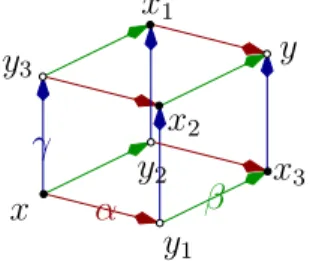
Integrability means that the system is3D-consistent [20, 10]:
Proposition 1.1.1. Consider a cube (x, y1, y2, y3, x1, x2, x3, y) with opposite faces holding the same discrete conformal structure ratios and the system, which given four valuesf(x), f(y1), f(y2), f(y3), solves for the four valuesf(x1), f(x2), f(x3) andf(y), withf a discrete holomorphic function (in the linear or quadratic frame- work). The system accepts a non trivial solution forf(y)if and only if the discrete conformal structure comes from parallelograms.
14 1. PRESENTATION OF SCIENTIFIC ACTIVITY
x
2x γ α β x
3y
2y
3y
x
1y
1Figure 1.5: The four values f(x), f(y1), f(y2), f(y3) determine uniquely f(x1), f(x2), f(x3) when f is discrete holomorphic, but f(y) is over-determined unless the weights come from parallelograms.
In this integrable case, the machinery of integrable systems gives us powerful tools, a zero curvature representation,Darboux-B¨acklundtransformations and isomonodromic solutions.
Our main results in this respect was to unify the linear and quadratic cases in the same framework, and to recoverKenyon’s result [71] giving theGreenfunc- tion of the discrete Laplacian in the rhombic case as a linear combination of discrete exponential functions. We understood thisGreenfunction as an isomonodromic solution and gave interesting properties of the discrete exponential functions [10].
When the diagonal ratios ρ are real numbers, or the cross-ratios q are uni- tary numbers, it implies that these quadrilaterals are rhombi, where even more interesting features appear: primitives of holomorphic functions can be defined.
This real integrability condition has been singled out by Duffin [60] in the context of discrete complex analysis, and by Baxter [30] as Z-invariant Ising model [24, 25, 42, 95].
In my thesis, I called this configurationcriticalfor this link with exactly solvable models and RichardKenyoncalled itisoradial for its link with circle patterns [71, 55].
Notice that Bazhanov, Mangazeev and Sergeev make a connection be- tween theIsingmodel and circle patterns in [32].
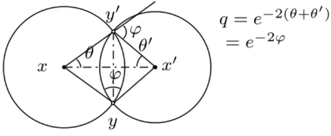
The cross-ratio preserving maps are closely related to the circle patterns idea [36, 98, 73, 43]. In this framework, proposed byThurston, a discrete conformal struc- ture is defined by a pattern of intersecting circles. A holomorphic function is defined by another circle pattern of the same combinatorics such that a pair of intersecting circles is mapped to another pair of circles, intersecting at the same angle. A quadri- lateral is defined for such a pair, defined by the two centers and the two points of intersection. The cross-ratio of these four points is given by the intersection angle.
Therefore circle patterns is a special case of cross-ratio preserving maps. Circle packings are a limit case of circle patterns with tangential adjacencies. In circle pattern theory, the discrete conformal parameters come from kite quadrilaterals, with orthogonal diagonals. Integrability meaning parallelism of opposite sides is then associated with rhombic embedding, that is to say isoradial circle patterns.
This way, a dual isoradial circle pattern emerges from the intersection points of the primal circle pattern, associated with the inverse cross-ratios.
Another way to view the 3D-consistency condition is to split the cube in two hexagons, the compatibility conditions are the same in both cases, see Fig. 1.8.
−→
Figure 1.6: Pairs of patterns of intersecting circles are a discrete conformal map when the intersection angles are pair-wise preserved.
= e
−2ϕθ
′ϕ
ϕ q = e
−2(θ+θ′)x
y y
′x
′θ
Figure 1.7: The cross-ratio of the centers and intersection points of two circles is given by their intersection angle.
β
x
3y
2y
3x
2y
x
3x y
2y
3x
2γ ≃
α
y
1x
1y
1x
1Figure 1.8: The six values f(x1), f(x2), f(x3), f(y1), f(y2), f(y3) over-determine the valuesf(x) andf(y) forf a discrete holomorphic function. The compatibility conditions on these six values are the same in both cases if and only if the discrete conformal structure comes from parallelogram sidesα, β, γ.
1.1.3. Exactly Solvable Models in Statistical Mechanics. The notion of integrability has several related meanings depending on the context. In statis- tical mechanics, its means that a thermodynamic continuous limit can be taken and it usually comes from aYang-Baxter equation. A finer notion iscriticality where this continuous limit is special, exhibiting a phase transition. In exactly solvable models, interesting critical systems, like the Ising model or its A-D-E - generalizations [47, 86], have a conformal continuous limit, in particular some 2- point correlation functions decay not exponentially fast with the distance between
16 1. PRESENTATION OF SCIENTIFIC ACTIVITY
the two points but as a power law (seeLanglands, Lewis and St Aubin [76]).
More generally, an observable depends not on the detail of the surface with marked points but more specifically on its conformal class. It was a goal of my PhD advisor Daniel Bennequinto find in the discrete setup of critical models what remained of Belavin, PolyakovandZamolodchikov conformal blocks.
I made advances in this program for the Ising model: I proved in my the- sis [16, 17] that the geometric condition of (real) integrability, already singled out by Baxter as Z-invariant Ising model [31], pinpointed the fact that a special observable in theIsing model, the fermionψx,y, became a discreteDiracspinor, a discrete holomorphic analog of √
d z. This is why I named this configuration critical.
In Australia, in collaboration with Paul A.Pearce, I investigated other statis- tical models, with the view to try and understand them in the framework of discrete Riemannsurfaces [12, 13, 14, 15]. We identified the integrable conformal twisted boundary conditions, on surfaces with boundary or as seams inserted in a closed surface along a loop, in several exactly solvable statistical models. We begun with the parafermionsZk[15], we investigated the relation between such twisted bound- ary conditions in conformal field theory [90, 89, 91, 51] and their lattice realization forA-D-E models [14], and understood it in the framework of the Thermodynamic Bethe-Ansatz[13]. We entangled in the fusion procedure the contribution of dif- ferent nodes in the Ocneanu graph [85] and clarified a correspondence between the nodes of theOcenanu graphs and our twisted discrete seams [12], ending up with a discrete version of the Vertex Operator Algebra governing the fusion rules.
Unfortunately, I didn’t succeed in making the connection between chirality, present in our twisted conformal boundary conditions, and discrete holomorphic/anti- holomorphic conformal blocks. What I missed was a clearer notion of discrete fiber bundle, more elaborate than the simple double-cover of spinors that I constructed by hand. I saw that the parafermion theory would have worked in a similar way but didn’t pursue in this direction, having enough on my hands with the development of the theory of discreteRiemannsurfaces in the framework of Discrete Differential Geometry. And what begun as a tool to tackle a problem in statistical mechanics ended up being my primary object of study.
Other researchers, independently or not, picked up similar ideas and discrete holomorphic functions theory was applied to statistical mechanics, by Costa- Santosand McCoy [53, 54] for higher genusIsing and dimer models, by Ra- jabpourandCardy[93] for discrete holomorphic parafermions,de Tili`ereand Boutillier [41, 42] for the Z-invariantIsing model and dimers, and Smirnov and Chelkak [102, 103, 48] for conformal invariance of percolation and more generally in 2D lattice models, making the link with hard-core probability theory like loop-erased random walks [77].
1.1.4. Topology. Our interest for a discrete version of conformal blocks takes its root in topology: The Verlindeformula governs the compatibility of the di- mensions of these blocks under fusion rules. This essentially finite information can be used to build topological invariants like knots invariants. Daniel Bennequin idea was that a discrete version of conformal blocks for statistical mechanics would have saved the trouble to go, from an exactly solvable model, to a conformal theory, back to the discrete data of its fusion rules [33].
Figure 1.9: A 1-1-correspondence between edge signed planar graphs and regular projections of links helps to manipulate and beautifully draw knots.
This interest in low dimensional topology came from my Diploma, conducted by Daniel Bennequin, in Strasbourg, where I showed the equivalence between Singertheorem onHeegaarddiagrams andKirbytheorem onDehnsurgeries.
This led to a long lasting interest in knot theory and its popularization, with (non peer reviewed) articles in the press [5, 9, 18, 19], with conferences addressed to the general public, specialized courses to draw nice knots and a popular web- sitehttp://entrelacs.net(see Fig. 1.9).
1.2. PhD supervision
I am co-advising the thesis of Fr´ed´eric Rieux, together with Pr Christophe Fiorio. Fr´ed´eric is beginning his second year and I am going to summarize the goals of his thesis and his first promising results.
The main goal is to be able to recognize as set of points in an Rn as a dis- cretization of a manifold. Our idea is to define a diffusion process and analyze it, in order to guess the correct dimension by the diffusion speed, and local geometry.
Once this identification is done, we use the local homogeneous coordinates to dis- cretize usual differential geometry and perform discrete analysis, derivation with estimation of tangents, of curvature, and so on.
1.2.1. Diffusion processes. Heat kernel or random walks have been widely used in image processing, for example lately bySun, OvsjanikovandGuibas[105]
and Gebal, Bærentzen, AanæsandLarsen[63] in shape analysis. It is indeed a very precious tool because two manifolds are isometric if and only if their heat kernels are the same (in the non degenerate case).
The heat kernelktof a manifoldM maps a couple of points (x, y)∈M×M to a positive real numberkt(x, y) which describes the transfer of heat fromy to xin timet. Starting from a (real) temperature T onM, the temperature after a time t at a pointxis given by
Htf(x) = Z
M
f(y)kt(x, y)dy.
The distance can be recovered from the heat kernel:
d2M(x, y) =−4 lim
t→0tlogkt(x, y).
The heat equation drives the diffusion process, the evolution of the temperature in time is governed by the (spatial)Laplace-Beltramioperator ∆M:
18 1. PRESENTATION OF SCIENTIFIC ACTIVITY
∂f(t, x)
∂t =−∆Mf(t, x).
It implies that if the eigenvalues of the Laplacian are sp(∆M) = {λi}i∈N, associated with eigenvector functionsφi, then the heat kernel is
kt(x, y) =X
i
e−λitφi(x)φi(y).
1.2.2. Discrete Laplacian. The first issue to use these ideas in the discrete setup is to define a good discrete Laplacian, or equivalently, a good diffusion process.
This diffusion process should be reasonably robust to noise, to outliers (points which are added by mistake) and to missing data.
This situation is understood in the realm of polyhedral surfaces and triangula- tions, and a time appraised discrete Laplacian, based on sound theoretical grounds is known for a long time, the so-calledcotangent weights Laplacian [92], which is the same as the one we talked about in the framework of discreteRiemannsurfaces:
∆f(x) = X
(x,xi)∈Γ1
ρ(x, xi) f(xi)−f(x)
whereρ(x, xi) = 1
2 cotanx\ixi−1x+ cotanxx\i+1xi
= d(yi+1, yi) d(xi, x)
with the triangle angles, the intrinsic metric computed on the flattened triangles pair andyi the center of the circumcircle to the triangle (xi, x, xi−1), similarly for yi+1, as depicted in Fig. 1.10.
x
i+1x
i−1y
ix
iy
i+1x
Figure 1.10: The diagonal ratiod(yd(xi+1,yi)
i,x) is the mean of the cotangents of the angles atxi−1 andxi+1.
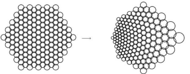
1.2.3. Digital Geometry. But the situation in Digital Geometry is somehow different, the data that is produced by a 3D-scanner is composed of a set of voxels (cubes in Z3) that samples the underlying continuous object. How can a good diffusion process be defined on such a locally rigid geometry?
We first studied a random walk based on the celebrated short-sighted drunk- ard’s walk, with equiprobability, no memory and no long range decision, the walker goes from a voxel cube, equiprobably to one of its 2dvertices, and then equiprobably to one of the available voxel of the object adjacent to it.
1/4 1/4
1/4 1/4
1/2 1/2
1/2 1/2
1/2 1/2 1/2 1/2
1 2 1
Figure 1.11: 2n walkers on a line inZ2 recover the binomials np .
1 4 1
2 1 4
(a) 4-4
1 8
3 4
1 8
(b) 8-8
1 8
5 8
1 4
(c) 8-4
1 4
5 8
1 8
(d) 4-8
Figure 1.12: There are only four local masks appearing on an 8-connected line in the first octant.
We begun with a discrete curve in Z2. We showed that for this process on a discrete line [94], the probability to find the walker at a certain point y, at a (discrete) timet, having begun atxis equivalent (for larget) to a normal distribu- tion √1
2πσe−d(x,y)2/2σ2 with the dispersionσ(t) increasing over time (proportional to√
t). It is a direct application of the Central Limit Theorem, our process being ergodic and similar patterns being repeated with a well defined probability. The same kind of argument will work in any dimension.
Unfortunately this dispersion depends on the slope of the line because 8- connected pixels act as bottle-necks compared to 4-connected pixels (see Fig.1.13).
1.2.4. Fuzzy set. Conductivity in crystals led me to think abouttunnel effect transition in quantum mechanics, where electrons can leap from a conductor to another. So we naively tried afuzzytransition, allowing walkers to wander one step away from the discrete line, on a thickened line with ghost pixels, in the 4-connected or 8-connected directions, projecting them back, later on, to the underlying line (see Fig. 1.14). This fuzzy diffusion is slower than the original one.
We have two parameters to play with, the allowed probabilities associated with 4 and 8 new neighbors. We optimized these probabilities in order to have a minimum deviation among the deviations for different slopes. This minimum is reached when 4 and 8-connected ghost pixels are both half as probable as the genuine pixels.
So beginning from a set of pixels, we add its 4 and 8-connected neighbors, with decreased probability, setup our random walk, and read from the weights of this process the adaptive distances between our points and integrate it into a curvilinear abscissa on our set.
20 1. PRESENTATION OF SCIENTIFIC ACTIVITY
46
Figure 1.13: Deviations of a typical mask on two hundred discrete lines of increasing slopes in the first octant. The minimum is reached for lines of slope 1 with only 8-connected pixels.
k
t0
t
Figure 1.14: Fuzzy segment withghost 4 and8 - connected pixels, which are pro- jected onto the underlying line.
50 100 150 200
48.2 48.9
45.4 49.6
46.1 50.3
46.8
5 10 15 20 25 30
34
29.1 31.2
27.7 32.6
29.8 31.9
28.4 30.5
Figure 1.15: Deviations for different lines using the curvilinear abscissa on the thin line and on the fuzzy line for optimized parameters.
The optimization procedure is there to insure that this process, when done on discrete lines, end up with what we should expect, that is to say a normal law with respect to the Euclidean distance inR2. So if the set is modeled on a curve, with feature size much lower than the size of discretization, a size of averaging mask large enough but lower than this feature size should recover the local geometry of the curve.
In order to denoise a function defined on the set, we simply convolve it with a certain power of the diffusion process. This power can be adaptive: large in flat
areas and small in tormented areas with small local feature size. The diffusion could be as well tailored in order to be non symmetric near sharp features to be preserved.
1.2.5. Discrete derivatives. Once this diffusion mask is defined, we use it to do numerical analysis on digital curves, computing derivative of functions such as tangency and curvature.
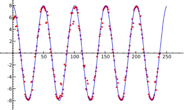
Consider the connected discretized graph of a function as a discrete curve in Z2. By applying the previous method, we are able to compute derivatives of this function by applying discrete derivative masks and convolving with our averaging kernel with a remarkable accuracy, as illustrated in Fig. 1.16 and 1.17.
50 100 150 200 250
-8 -6 -4 -2 2 4 6 8
Figure 1.16: Estimation of the discrete adaptive derivative function ofx7→sin(x) and the values of the real derivative functionx7→cos(x), computed according to a mask of length 15 on a sample of 250 points.
25 50 75 100 125 150 175
-8 -6 -4 -2 2 4 6 8
Figure 1.17: Comparison between the estimation of the second order derivate of x7→sin(x) and the real values, computed with a mask of length 20 and a sample of 400 points.
Discrete Riemann Surfaces
2.1. Conformal maps
Before discretizing conformal maps, it is good to recall what holomorphic and analytic functions are in a visual way, helping to build intuitions and pictures of how the discrete version should behave. This section illustrates this point using a software tool that I have programmed for pedagogical reasons and with which I have produced an article in the CNRSImages des math´ematiques [3].
Everybody is used to visualizing a function from the plane to the real numbers, like precipitation maps (see Fig. 2.1): simply color the target spaceRwith colors and plot each point (x, y) of the domain space R2 by the color f(x, y). Exactly
vv v
vv v
vv v
vv v v
vv v
vv v
vv v
vv v
Hauteur totale des précipitations
(millimètres)
1000 900 800 700 600 500 400 300 250 200 175 150 125 100 75 50 25 0
Figure 2.1: Precipitation map in France for July 2009. The color indicates a real value according to the scale. cM´et´eo France
the same can be done with complex valued functions: choose a picture to cover the complex plane seen as the target space, and visualize the functionf : C→C by coloring the pointz∈C with the colorf(z).
23
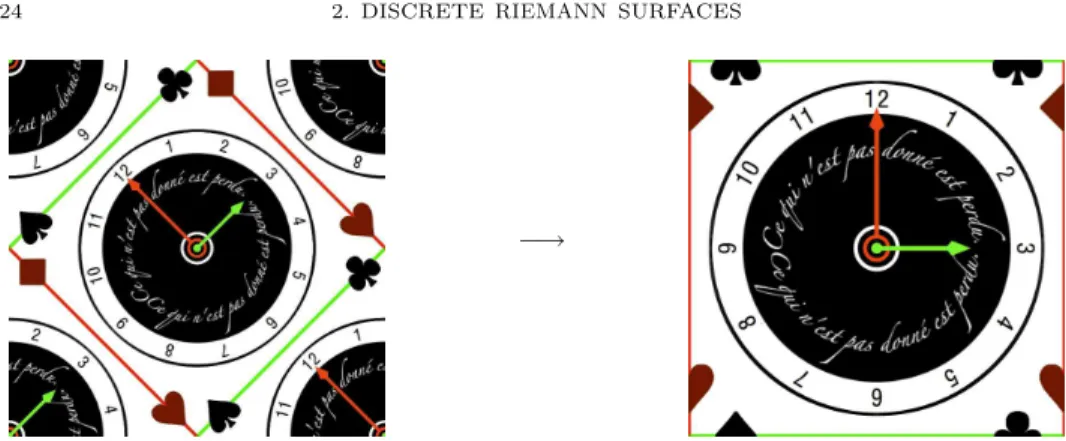
24 2. DISCRETE RIEMANNSURFACES
−→
Figure 2.2: The similitudez7→(1 +i)z pictured as the pull-back of the picture of a clock paving the complex plane.
The complex differentiability is visualized by the fact that the picture in the domain space, away from singularities, is to the first order around z, a simple similitude of parameter 1/f′(z) since locally, the function behave as f(z+z0) = f(z0) +z×f′(z0) +o(|z|). In particular, the zeros of the derivative are very easy to spot since the similitude ratio tends to infinity. There, the function is no longer conformal, it behaves locally as a monomial,f(z+z0)−f(z0) = f(k)k!(z0)zk+o(zk) and the angles throughz0 are divided byk, replicating the featuresk times.
Figure 2.3: The graph of a polynomial and of the monomialz7→z3.
The forward image of a picture by a holomorphic function is much more difficult to obtain, because such a function is not injective, it has a definite degree k and every non critical value inC is attained exactlyk times (see Fig. 2.4).
Although I do have a notion for polynomials in the integrable case, I don’t have a good discrete notion for its zeros. The issue is that a zero of high order is difficult to place inside a polygon: since z 7→ zk folds k times the plane onto itself, the polygon must have many vertices so that its polygonal image windsktimes around the origin. Since we are mainly concerned with quadrilaterals, it is only possible to wind once, zero or minus once around a point, allowing for only one degree of zero and pole, with the extra possibility of degeneracy. Higher degree zeros are seen as
Figure 2.4: The direct images by the squarez7→z2and the cubez7→z3are blurry, every point is the image of two, resp. three points. They are the pull-back of the multi-valued functions square and cubic roots.
clusters of simple zeros. Another option would be to supplement the values of a function at vertices by integer valued tags.
The integrability of the parallelogram case allows for the expansion of discrete holomorphic functions in series of whether discrete exponentials or discrete poly- nomials [11].
Together with a student from India, LalitSirsikarfrom the Institute of Tech- nology, Banaras Hindu University, we programmed a java applet∗ based on my previous work with the Java Tools for Experimental Mathematics library† devel- oped by the Technical University Berlin team in which I belonged. This applet lets the user write an expression for a holomorphic function f(z), shows a picture in the target space, as a single tile in a window, its pull-back deformed picture in the domain space in another window. In this domain space, two draggable points, a red and a blue, drive two complex numbers,z0 and z1. Their imagesf(z0), f(z1) by the function f are plotted in the target space, as two points, mapped back to the fundamental tile. Aweb-cam version is as well available, where the picture of the people standing in front of the computer is continuously deformed. I use this applet during special public events and it is very successful with students.
These two points are linked by a polygonal line corresponding to the sequence of Taylorpolynomials off atz0,
Sn(z1) =f(z0) + (z1−z0)f′(z0) +· · ·+(z1−z0)n
n! f(n)(z0)
expressed as a function ofz1. When theTaylor series converges, this polygonal line spirals towards f(z1), when it diverges, the polygonal lines exhibit different interesting behaviors. A third window shows the pull-back by the last computed Taylor polynomial and the disk of convergence of the series is in general very apparent visually as a zone resembling the domain space. This can be probed by moving the blue point in the domain space and witnessing whether the series seems to numerically converge or not, the last bluish point of the polygonal line corresponding to the value of the partial sum in Fig. 2.6. The inversion z 7→1/z
∗http://www.math.univ-montp2.fr/SPIP/IMG/jar/ComplexImage.jar
†Java Tools for Experimental Mathematics: http://jtem.de
26 2. DISCRETE RIEMANNSURFACES
−→
Figure 2.5: The graph of the tangent functionz7→tan(z), on the left, the red point z0 and the blue pointz1 in the domain space, with the converging polygonal view of the partialTaylorsums, fromf(z0) tof(z1), mapped back to the fundamental tile in the target space.
Figure 2.6: The graph of the 8th Taylor polynomial of the tangent function z 7→ tan(z), expanded at the red point z0. The disk of convergence of the series is already discernible as the zone where the difference with Fig. 2.5 is visually not significant.
preserves globally the unit circle, sending inside out, especially exchanging the origin and the infinity. It is a M¨obius transformation, sending circles to circles, except circles through the origin which are exchanged with lines (such as the red and green axis lines), see Fig. 2.7. Higher order poles z 7→ 1/zk are no longer M¨obiustransformations.
Together with polynomials, they form the field of rational fractions. I don’t have a good notion for localized poles and their discrete counterparts don’t form a canonical field, neither for the multiplication, nor for the composition, without making arbitrary choices.
Figure 2.7: The inversionz7→1/z and a higher degree polez7→1/z2.
Theexponential function is unwrapping centered circles and their rays to ver- tical and horizontal lines because x+i θ 7→ rexp(iθ) where r = exp(x) is the radius of the circle, image of the vertical line at real part x. The exponential is 2iπ-periodic. Its reciprocal, the logarithm, is not even a function because it is multi-valued. Given a determination, one has to adjust the vertical size of the tiles to divide 2iπ so that the discontinuity of the tiling synchronizes with the jumps in the determination, giving the illusion of a continuous function, which wraps the horizontal and vertical lines to centered circles and their rays (see Fig. 2.8), showing a logarithmic singularity at the origin. Both notions can be discretized, leading to discrete exponentials and thediscrete Greenfunction.
Figure 2.8: The exponential and the logarithm.
The resulting image is invariant under some rotations because the target space is a lattice whose vertical period divides 2iπ. But the horizontal period λof the lattice translates to the invariance by homothecy. One can take as a basis of the lattice not (λ,2iπ) but (λ+ 2ikπ,2iπ), linking rotation and homotecy, obtaining nicespirals like in Fig. 2.9.
Beyond zeros of the derivative, poles and logarithmic singularities, anessential singularity is an accumulation point of zeros or poles, like in Fig. 2.10.
28 2. DISCRETE RIEMANNSURFACES
Figure 2.9: The complex logarithmz7→log(z)×(1 +µ i) for appropriateµ∈R.
Figure 2.10: The essential singularity of the function z7→ exp(1/z) at the origin, with accumulations of zeros on the negative real side and accumulation of poles on the positive real side.
2.2. Real discrete conformal structure
We begin our discussion of Discrete Complex Analysis by the case when quadri- lateral dual diagonals are orthogonal, what I call areal discrete conformal structure.
2.2.1. Graphs and Discrete Conformal Structure. Let♦ a cellular de- composition of an oriented surface by quadrilaterals, that is to say a set ♦0 of vertices, linked by a set ♦1 of edges, themselve belonging to four-sided faces ♦2. Every edge is attached at most twice to faces. An edge attached only once is a boundary edge, twice is aninterior edge. If the boundary is empty, the surface is closed.
We suppose that every loop is of even length (it is the case for trivial loops).
Therefore the graph is bipartite and it defines two dual locally planar graphs Γ
and Γ∗, by their vertices ♦0 = Γ0⊔Γ∗0, their edges (x, x′)∈ Γ1 and (y, y′)∈ Γ∗1, diagonals of the quadrilaterals (x, y, x′, y′)∈♦2. In the closed case, this forms faces Γ2≃Γ∗0, Γ∗2≃Γ0. The boundary case can be handled similarly.
y
′y
x
′x
Figure 2.11: Dual edges (x, x′)∈Γ1and (y, y′)∈Γ∗1are diagonals of a quadrilateral (x, y, x′, y′)∈♦2.
We call the data of a graph Γ, whose unoriented edges are equipped with a positive real number a discrete conformal structure and for e ∈ Γ1, we note ρ(e)>0.
We equip the dual graph of positive numbers in the following fashion: In the quadrilateral (x, y, x′, y′)∈♦2, we give to the dual edge (y, y′) = (x, x′)∗∈Γ∗1 the positive real constantρ(y, y′) = 1/ρ(x, x′). This number is to be understood later on as the ratio of dual diagonals lengthsρ(x, x′) = ℓ(y,yℓ(x,x′′)).
For commodity, we define Λ := Γ⊔Γ∗thedoublegraph. The duality exchanges Γk and Γ∗2−k, therefore is a bijection in Λ and ρ is defined on Λ1 such that, for e∈Λ1,ρ(e∗) = 1/ρ(e).
2.2.2. Complexes. We recall elements of de Rham cohomology: We define the complex ofchains as the vector spaces spanned by vertices, edges and faces, for each of the above graphsC(G,R) =C0(G,R)⊕C1(G,R)⊕C2(G,R). We identify change of orientation of cells and negation of coefficient: for e∈ Λ1 and λ ∈ R, λe¯=−λ e∈C1(Λ,R) is a 1-chain. The 0-chainsC0(♦,R) are related to the other 0-chainsC0(♦,R)≃C0(Λ,R). For 0≤k≤2,Ck(Λ,R)≃Ck(Γ,R)⊕Ck(Γ∗,R), withCk(Γ,R)≃C2−k(Γ∗,R) through Poincar´eduality.
These complexes are equipped with aboundaryoperator∂G:Ck(G)→Ck−1(G), null on vertices, difference of end-points∂G(a, b) =b−aon an edge, and sum of the oriented edges forming the boundary of a face. It fulfills ∂G2 = 0. The ker- nel ker∂G =:Z•(G) of the boundary operator are theclosed chains or cycles. Its image are the exact chains. It provides the dual spaces of forms, called cochains, Ck(G) := Hom(Ck(G),R) with a coboundary dG :Ck(G)→ Ck+1(G) defined by
30 2. DISCRETE RIEMANNSURFACES
Stokesformula:
Z
(x,x′)
dGf :=f(∂G(x, x′)) =f(x′)−f(x), Z Z
F
dGα:=
I
∂GF
α.
Acocycle is a closed cochain and we noteα∈Zk(G) whendGα= 0.
We will drop the mention of the graph when there is no possible confusion or when the difference is not essential; we can indeed identify closed forms on different graphs under certain conditions:
x x
x
1x
2y
2y
1y
dx
d(2.1) (2.2)
y y
′x
′Figure 2.12: Notations.
2.2.3. Averaging forms. A form on ♦ can be averaged into a form on Λ:
This map A from C•(♦) to C•(Λ) is the identity for functions of vertices and defined by the following formulae for 1 and 2-forms:
Z
(x,x′)
A(α♦) := 1 2
Z
(x,y)
+ Z
(y,x′)
+ Z
(x,y′)
+ Z
(y′,x′)
α♦, (2.1)
Z Z
x∗
A(ω♦) := 1 2
d
X
k=1
Z Z
(xk,yk,x,yk−1)
ω♦, (2.2)
where notations are made clear in Fig. 2.12.
The mapAis neither injective nor surjective in the non simply-connected case.
Its kernel is Ker (A) = Vect (d♦ε), whereεis thebiconstant, yielding +1 on Γ and−1 on Γ∗.
Proposition 2.2.1. Averaging carries cocycles on ♦to cocycles on Λ and its image are the cocycles ofΛ verifying that their holonomies along cycles of Λ only depend on their homology on the combinatorial surface
2.2.4. Hodge star. TheHodgestar, in the continuous theory of surfaces is defined on 1-forms, in an orthonormal local coordinates (x, y), by∗(f dx+g dy) =
−g dx+f dy. In the discrete case the duality transformation plays the role of rotating the orthogonal (x, y) coordinates and the discrete conformal structure takes care of the norm, leading to the following definition:
(2.3)
Z
e∗∗α:=ρ(e) Z
e
α
A 1-form α ∈ C1(Λ) is of type (1,0) if and only if, for each quadrilateral (x, y, x′, y′)∈♦2,R
(y,y′)α=iρ(x, x′)R
(x,x′)α, that is to say if∗α=−iα. We define similarly forms of type (0,1) with +iand−iinterchanged. A form isholomorphic, resp. anti-holomorphic, if it is closed and of type (1,0), resp. of type (0,1). A functionf : Λ0→C is holomorphic iffdΛf is. This condition can be rewritten f is holomorphic ⇐⇒ ∀(x, y, x′, y)∈♦2, f(y′)−f(y) =iρ(x, x′) f(x′)−f(x)
. We note Ω(Λ) the space of holomorphic forms.
2.2.5. Wedge product. We construct a wedge product on♦such thatd♦ is a derivation for this product ∧: Ck(♦)×Cl(♦)→ Ck+l(♦). It is defined by the following formulae, forf, g∈C0(♦),α, β∈C1(♦) andω∈C2(♦):
(f·g)(x) :=f(x)·g(x) forx∈♦0, Z
(x,y)
f·α:=f(x) +f(y) 2
Z
(x, y)α for (x, y)∈♦1, Z Z
(x1,x2,x3,x4)
α∧β:=1 4
4
X
k=1
Z
(xk−1,xk)
α Z
(xk,xk+1)
β− Z
(xk+1,xk)
α Z
(xk,xk−1)
β Z Z
(x1,x2,x3,x4)
f ·ω:=f(x1)+f(x2)+f(x3)+f(x4) 4
Z Z
(x1,x2,x3,x4)
ω for (x1, x2, x3, x4)∈♦2.
The exterior derivatived♦is a derivation for the wedge product, for functions f, g and a 1-formα∈C1(♦):
d♦(f g) =f d♦g+g d♦f, d♦(f α) =d♦f∧α+f d♦α.
We define anheterogeneous wedge product for 1-forms living on diagonals Λ1, as a 2-form living on faces♦2. The formula is:
Z Z
(x,y,x′,y′)
α∧β:= 1 2
Z
(x,x′)
α Z
(y,y′)
β− Z
(y,y′)
α Z
(x,x′)
β
(2.4)
Together with theHodge star, they give rise, in the compact case, to the usual scalar product on 1-forms:
(2.5) (α, β) :=
Z Z
♦2
α∧ ∗β¯= (∗α,∗β) = (β, α) = 12 X
e∈Λ1
ρ(e) Z
e
α Z
e
β¯