HAL Id: hal-00004901
https://hal.archives-ouvertes.fr/hal-00004901v4
Submitted on 12 Oct 2006
HAL is a multi-disciplinary open access archive for the deposit and dissemination of sci- entific research documents, whether they are pub- lished or not. The documents may come from teaching and research institutions in France or abroad, or from public or private research centers.
L’archive ouverte pluridisciplinaire HAL, est destinée au dépôt et à la diffusion de documents scientifiques de niveau recherche, publiés ou non, émanant des établissements d’enseignement et de recherche français ou étrangers, des laboratoires publics ou privés.
Distribution of resonances for open quantum maps
Stéphane Nonnenmacher, Maciej Zworski
To cite this version:
Stéphane Nonnenmacher, Maciej Zworski. Distribution of resonances for open quantum maps. Com- munications in Mathematical Physics, Springer Verlag, 2007, 269 (2), pp.311-365. �10.1007/s00220- 006-0131-0�. �hal-00004901v4�
ccsd-00004901, version 4 - 12 Oct 2006
ST´EPHANE NONNENMACHER AND MACIEJ ZWORSKI
1. Introduction
1.1. Statement of the results. In this paper we analyze simple models of classical chaotic open systems and of their quantizations. They provide a numerical confirmation of the fractal Weyl law for the density of quantum resonances of such systems. The exponent in that law is related to the dimension of the classical repeller of the system. In a simplified model, a rigorous argument gives the full resonance spectrum, which satisfies the fractal Weyl law. Our model is similar to models recently studied in atomic and mesoscopic physics (see §2.4 below). Before stating the main result we remark that in this paper we use mathematicians’ notationhfor what the physicists call~. That is partly to stress that ourhis a small parameter in asymptotic analysis, not necessarily interpreted as the Planck constant.
Theorem 1. There exist families of symplectic relations, Be ⊂ T2 ×T2, and of their (subunitary) quantization, Beh ∈ L(CN), N = (2πh)−1, such that
#
λ∈Spec(Beh) : |λ| ≥r =c(r)h−ν +o(h−ν), r >0, h =hk = (2πDk)−1 →0, k→ ∞, ν= dim Γ−(B)e ∩W+(B)e
, c(r) = (2π)−νχ[0,r
0(B)]e (r), 0< r0(B)e <1,
where the integer parameter D > 1 depends on B. The sete Γ−(Be) ⊂ T2 is the forward trapped set of Be and W+(B)e is the unstable manifold of Be at any point of Γ−(Be). The eigenvalues are counted with multiplicities.
In the model discussed in detail we took D = 3. The asymptotics are actually much more precise and include uniform angular distribution (see Prop. 5.5). The resonances lie on a lattice, and some of this structure is also seen in numerically computed more generic situations (some numerical results have been presented in [40, 38, 39]). Each symplectic relation Be (or “multivalued symplectic map”) is defined together with the probabilities, for any point, to be mapped to each of its images: Be thus represents a certain stochastic process. The quantizationsBeh quantize the relations together with their jump probabilities in the precise sense given in §4.4.
1
In the models used in Theorem 1 we can compute the conductance and the shot noise power (or the closely related Fano factor) — see§2.4.3 and references given there for physics background and §6 for precise definitions.
Theorem 2. Suppose that the models in Theorem 1 have the openings consisting of two
”leads” of equal width (see §6.1 for a detailed description), so that each lead carries the same number, M(h) ∼h−1, of scattering channels. Then, the quantum conductance (6.2) between the two leads satisfies
(1.1) g(h) = 1
2M(h) 1 +o(1)
, h=hk →0. The Fano factor (6.3) is given by
(1.2) F(h) = 11
80
M(h)ν
g(h) 1 +o(1)
, h=hk →0, where the exponent ν is the same as in Theorem 1.
The theorem should be interpreted as follows. In (1.1) we see that for a model of scattering through a chaotic cavity, approximately one half of the scattering channels get transmitted from one lead to the other, the other half being reflected back (this is natural and well known). Asymptotics in (1.2) are more interesting. We see that the fractal Weyl law, h−ν, appears in the expression for the Fano factor. In the interpretation of the Fano factor in terms of “shot noise” (see §2.4.3), 11/80 gives the average “shot noise” per
“nonclassical transmission channel”. This number is close to the random matrix theory prediction for this quantity, namely 1/8 [26, 57]. In fact, had (1.2) come from a physical experiment rather than an asymptotic computation, it would be regarded as being in a very good agreement with random matrix theory1.
Much of the paper is devoted to rigorous definitions of the objects appearing in the statements of the two theorems. In this section we give some general indications, with detailed references to previous works appearing below.
We consider the two-torus T2 = [0,1)×[0,1) as our classical phase (with coordinates ρ = (q, p)). Classical observables are functions on T2 and classical dynamics is given in terms of relations, B ⊂T2×T2, which are unions of truncated graphs of symplectic (area and orientation preserving) maps T2 →T2. An example is given by the baker’s relation (1.3) (ρ′;ρ) = (q′, p′;q, p)∈B ⇐⇒
q′ = 3q , p′ =p/3, 0≤q ≤1/3 q′ = 3q−2, p′ = (p+ 2)/3, 2/3≤q <1. This is a “rectangular horseshoe” modeling a Poincar´e map of a chaotic open system: some points (here {ρ : 1/3< q <2/3}) are thrown out “to infinity” at each iteration.
1We are grateful to Yan Fyodorov for this amusing comment.
For relations such as B we can define the forward and backward trapped sets (see (2.4) for the definition in the case of flows):
ρ∈Γ− ⇔ ∃{ρj}∞j=0, ρ0 =ρ , (ρj;ρj−1)∈B , j >0, ρ∈Γ+ ⇔ ∃{ρj}0j=−∞, ρ0 =ρ , (ρj;ρj−1)∈B , j ≤0.
In the example (1.3), Γ− =C×[0,1), Γ+ = [0,1)×C, whereC is the usual 13−Cantor set.
We also define thetrapped set K = Γ+∩Γ− and, at points of K, the stable and unstable manifolds,W±. In the case of the above baker’s relation,
ν= dim Γ−∩W+ = 1
2dimK = dim Γ+∩W− = log 2 log 3, but for general (possibly multivalued) relations these equalities do not hold.
A quantization (in the sense made rigorous in §4.5) of B is given by (1.4) Bh =FN∗
FN/3 0 0
0 0 0
0 0 FN/3
, h= (2πN)−1, 3|N , where FM is the discrete Fourier transform on CM.
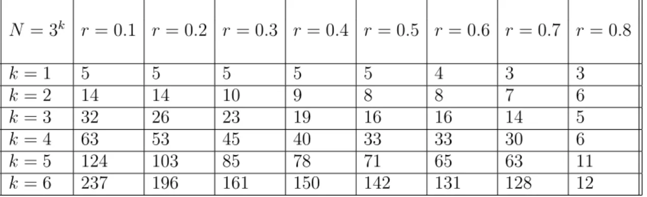
N = 3k r= 0.1 r = 0.2 r= 0.3 r = 0.4 r= 0.5 r= 0.6 r = 0.7 r= 0.8
k = 1 5 5 5 5 5 4 3 3
k = 2 14 14 10 9 8 8 7 6
k = 3 32 26 23 19 16 16 14 5
k = 4 63 53 45 40 33 33 30 6
k = 5 124 103 85 78 71 65 63 11
k = 6 237 196 161 150 142 131 128 12
Table 1. Number of eigenvalues of Bh in the regions{ |λ|> r}, for 2πh= 1/N, N given by powers of 3.
Table 2 shows the analogies between the eigenvalues of this subunitary quantum map and the resonances of a Schr¨odinger operator for a scattering situation (see §2.1).
For Bh given by (1.4) we are unable to prove the fractal Weyl law presented in the last line of Table 2, but numerical results strongly support its validity [40]. A striking illustration is given by tripling N, in which case the number of eigenvalues approximately doubles, in agreement with the fractal Weyl law — see Table 1.
The family of subunitary quantum maps in the main theorem is obtained by simplifying Bh, and is described explicitly in (5.2). It is a quantization of a more complicated multival- ued relation for which Γ+ =T2, Γ−=C×[0,1), and Γ−∩W+ ≃C — see Proposition 5.1.
Theorem 1 follows from the more precise Proposition 5.4.
1.2. Organization of the paper. In §2 we present related results from recent mathe- matical, numerical, and physics literature. In particular, in §2.4.3 we give the physical motivation for the objects appearing in Theorem 2 above. §3 is devoted to the review of classical dynamics used in our models, stressing the dynamics of open baker’s relations.
In §4 we first review the quantization of tori. We assume the knowledge of semiclas- sical quantization in T∗Rn (pseudodifferential operators) but otherwise the presentation is self contained. The definitions of Lagrangian states associated to smooth and singular Lagrangian submanifolds is based on the ideas of Guillemin, H¨ormander, Melrose, and Uhlmann in microlocal analysis but, partly due to technical differences, we give direct proofs of the properties we need in this paper. These properties are used to analyze the quantizations of the baker’s relation coming from the work of Balazs, Voros, Saraceno and Vallejos.
Numerical results for the (usual) quantization of the open baker’s relation have been presented in [40], we briefly summarize them in §4.6. In §5 we discuss the toy model Beh, with two different interpretations. That section contains the proof of Theorem 1.
Finally in §6 we give precise definitions of objects appearing in Theorem 2 and in a lengthy computation we give its proof.
Acknowledgments. We are grateful to Christof Thiele and Terry Tao for pointing out the
“Walsh” interpretation of our toy model, and to the anonymous referee for his comments.
The first author thanks Marcos Saraceno for his insights on that model, and Andr´e Voros for interesting questions. He is also grateful to UC Berkeley for the hospitality in April 2004. Generous support of both authors by the National Science Foundation under the grant DMS-0200732 is also gratefully acknowledged.
2. Motivation and background
In this section we discuss motivating topics in mathematics and theoretical physics, and survey related results.
2.1. Schr¨odinger operators. The original motivation comes from the study of resonances in potential scattering. The simplest case is given by considering the following quantum Hamiltonian:
(2.1) H =−h2∆ +V(q), V ∈ Cc∞(Rn;R).
By assuming that the potential vanishes near infinity and that it is infinitely differentiable, we eliminate the need for technical assumptions — see [22] and [53] for more general
settings, in the analytic and C∞ categories respectively. For instance, as noted in [50, (c.32)-(c.33)] the theory of [22] applies to arbitrary homogeneous polynomial potentials at nondegenerate energy levels.
h→0 N = (2πh)−1 → ∞
χexp −it(−h2∆ +V)/h
χ , t≥0, Bth,t = 0,1,· · · χ a cut-off on the interaction region Bh a subunitary matrix
e−itz/h,z a resonance of H =−h2∆ +V λt, λ an eigenvalue ofBh ∈ L(CN)
z ∈[E−h, E+h]−i[0, γh] 1≥ |λ|> r >0
#{z ∈[E−h, E+h]−i[0, γh]} ≃ C(γ)h−µE #{λ,|λ|> r} ≃ C(r)Nν Table 2. Analogies between Schr¨odinger propagators and open quantum maps.
Before discussing open systems we recall the well known results for closed systems, ob- tained for instance by considering H above on a bounded domain Ω ⊂ Rn and imposing a self-adjoint boundary condition at ∂Ω (Dirichlet or Neumann). Then the spectrum, Spec(H), of H is discrete and, at a non-degenerate energy level E its density is described by the celebrated Weyl law:
(2.2) #{Spec(H)∩[E−δ, E+δ]}= 1 (2πh)n
Z Z
|p2+V(q)−E|<δ
dq dp+O(h1−n), see [14, 25] and references given there. We note that this implies a precise upper bound (2.3) #{Spec(H)∩[E−Ch, E+Ch]}=O(h1−n),
which can be improved further by making assumptions on the classical flow of the Hamil- tonian p2 +V(q) on Ω, see [14, 25].
For open systems, with the simplest example given by the Hamiltonian in (2.1), real eigen- values are replaced by complex resonances. The simplest definition (easily made rigorous in the case (2.1)) comes from considering the meromorphic continuation of the resolvent.
Defining the Green’s function G(z, q′, q) for Imz >0 through (z−H)−1u(q′) =
Z
Rn
G(z, q′, q)u(q)dq , u∈ Cc∞(Rn),
then G(z, q′, q) admits a meromorphic continuation in z across the real axis. Its poles for Imz <0 (which do not depend on (q′, q)) are the quantum resonances of H.
Counting of resonances is affected by the dynamical structure of the scatterer much more dramatically than counting of eigenvalues of closed systems. Since we are now counting points in the complex plane we need to make geometric choices dictated by dynamical and physical considerations. Here we consider scatterers and energies exhibiting a hyperbolic classical flow, and regions in the lower half-plane which lie at a distance proportional to h from the real axis. This choice is motivated as follows. Quantum mechanics interprets a resonance at z = E−iγ in terms of a metastable state, which decays proportionally to exp(−tγ/h). Hence for γ ≫ h the decay is so rapid that the state is invisible. On the other hand, for many chaotic scatterers there are no resonances with γ ≪h. One class for which this is known rigorously consists in the Laplacian on co-compact quotients Hn/Γ, H =−h2∆Hn/Γ, when the dimension of the limit set satisfies δ(Γ)<(n−1)/2. This follows from the work of Patterson and Sullivan — see the discussion below and [37].
After a complex deformation (see [53] and references given there) the long living quantum states should semiclassically concentrate on the set of phase space points which do not escape to infinity, that is on thetrapped setKE defined as follows: let ΞH be the Hamilton vector field of the Hamiltonian H(q, p) =p2/2 +V(q):
ΞH = Xn
j=1
pj∂qj−∂qjV(q)∂pj. Then
KE
def= Γ+(E)∩Γ−(E), with the forward/backward trapped sets Γ±(E)def= {ρ∈ΣE : exptΞH(ρ)6→ ∞, ∓t→ ∞}.
(2.4)
Suppose that the flow generated by ΞH is hyperbolic near KE′ for E′ close to a non- degenerate energy E. That means that the field ΞH does not vanish on the energy surfaces ΣE′ ={p2+V(q) =E′} ⊂T∗Rn forE′ ≈E, and that forρ∈ΣE′ near KE′,
TρΣE′ =RΞH(ρ)⊕E+(ρ)⊕E−(ρ),
ΣE′ ∋ρ7−→E±(ρ)⊂TρΣE′ is continuous, d(exptΞH)(E±(ρ)) = E±(exptΞH(ρ)),
kd(exptΞH)(X)k ≤Ce±λtkXk, for all X ∈E±(ρ), ∓t≥0.
(2.5)
Weaker assumptions are possible — see [50, §5] and [53, §7].
Typically, the set KE has a fractal structure and in the semiclassical estimates the Minkowski dimension naturally appears:
dimKE = 2n−1−sup
c : lim sup
ǫ→0 ǫ−cvol{ρ∈ΣE : dist(KE, ρ)< ǫ}<∞ . We say that KE is of pure dimension if the supremum is attained. For simplicity of the presentation we assume that this is the case.
Under these assumptions the estimate (2.3) has an analogue for chaotic open systems [53]. ForC0 >0 there exists C1 such that
(2.6) #
Res(H)∩ {z : |z−E|< C0h} ≤C1h−µE, dimKE = 2µE+ 1. We notice that for a closed system the trapped set is the entire energy surface, so that in that case µE = n−1, hence (2.6) is consistent with (2.3). In this note we use open quantum maps to provide the first evidence that this precise estimate is optimal.
We should also mention that, as was already stressed in the work of Sj¨ostrand [50], the estimates involving the dimension are only reasonable when the flow is strictly hyperbolic.
In the case of more complicated flows the estimates should be stated in terms of properties ofescapeorLyapunovfunctions associated to the flow – see [50, 53]. For expository reasons the estimates involving the dimension are however most persuasive.
2.2. Survey of related results. The first indication that fractal dimensions enter into counting laws for quantum resonances of chaotic open systems appears in a result of Sj¨ostrand [50]:
#
Res(H)∩ {z : |z−E|< δ , Imz >−γ} ≤C1δ h
γ −n
γ−12me , Ch≤γ ≤1/C , max(h12, h/γ)≤δ≤2/C ,
(2.7)
whereme is any number greater than the dimension of the trapped set in the shellH−1(E− 1/C2, E+ 1/C2). In a homogeneous situation, such as for instance obstacle scattering, the dimension of KE, 2µE + 1, is independent of E, so that m >e 2(µE + 1).
The improvement in [53] quoted in (2.6) lies in providing a bound for the number of resonances in a smaller region D(E, Ch) ={z ∈C : |z−E|< Ch}. Heuristic arguments suggesting that the estimate (2.7) should be optimal were given in [31] and [32].
Another class of Hamiltonians with chaotic classical flows and fractal trapped sets is given by Laplacians on convex co-compact quotients, H/Γ. Here Γ is a discrete subgroup of isometries of the hyperbolic plane H, such that
• All elements γ ∈ Γ are hyperbolic, which means that their action on H can be represented as
α◦γ◦α−1(x, y) =eℓ(γ)(x, y), (x, y)∈H≃R+×R, α∈Aut(H). (2.8)
• Ifπ :H→H/Γ, and Λ(Γ)⊂∂H is the limit set of Γ, that is the set of limit points of {γ(z) :γ ∈Γ}, z ∈H, then π(convex hull Λ(Γ)) is compact.
The trapped set is determined by Λ(Γ): trapped trajectories are given by geodesics con- necting two points of Λ(Γ) at infinity, and
dimKE = 2δΓ+ 1, δΓ= dim Λ(Γ).
The limit set is always of pure dimension, which coincides with its Hausdorff dimension.
A nice feature of this model is the exact correspondence between the resonances of H =h2(−∆H/Γ−1/4),
and the zeros of the Selberg zeta function, ZΓ(s)2:
z ∈Res(H) ⇐⇒ ZΓ(s) = 0, z=h2(s(1−s)−1/4), Res ≤δΓ, (2.9)
where the multiplicities of zeros and resonances agree. The Selberg zeta function is defined by the analytic continuation of
ZΓ(s) = Y
{γ}
Y
k≥0
1−e−(s+k)ℓ(γ)
, Res > δΓ,
where {γ} denotes a conjugacy class of a primitive element γ ∈ Γ (an element which is not a power of another element), and we take a product over distinct primitive conjugacy classes (each of which corresponds to a primitive closed orbit). The length ℓ(γ) of the corresponding closed orbit appears in (2.8). The exact analogue of (2.6) is given by (2.10) #{s : ZΓ(s) = 0, Res >−C0, r <Ims < r+C1} ≤C2rδΓ,
which is a consequence of an estimate established by Guillop´e-Lin-Zworski [20] in a more general setting of convex co-compact Schottky groups in any dimension,
(2.11) |ZΓ(s)| ≤CKeCK|s|δΓ, Res ≥ −K , for any K.
This improved earlier estimates of [59], the proof of which was largely based on [50].
In the (non-quantum) context of rational maps on the complex plane, similar results were obtained concerning the zeros of associated zeta functions [11, 54]. Take f a uniformly expanding rational map on C (for instance z 7→ z2 +c, c < −2), and call fn its n-fold composition. The zeta function associated with this map is given by
(2.12) Z(s) = exp
− X∞
n=1
n−1 X
fn(z)=z
|(fn)′(z)|−s| 1− |(fn)′(z)|−1
.
2We refer to [42] for this and a general treatment. The term 14 in the definition of the Hamiltonian H comes from requiring that the bottom of the spectrum ofH is 0, so that Green’s function (H−λ2)−1 is meromorphic inλ∈C
Then the number or resonances in a strip is also given by a law of the type (2.10), where δΓ is replaced by the dimension of the Julia set:
J = [
n≥1
{z : fn(z) =z}. Note that this set is also made of “trapped orbits”.
2.3. Survey of numerical results. The first model investigated numerically was perhaps the hardest to give definitive results. Lin [30, 31] studied the semiclassical Schr¨odinger Hamiltonian (2.1) with a potential made of 3 Gaussian “bumps”. The semiclassical res- onances were computed using the method of complex scaling and were counted in boxes of type [E − δ, E + δ] − i[0, h] with δ fixed. The purpose was to verify optimality of Sj¨ostrand’s estimate (2.7) with these parameters. The results were encouraging but not conclusive. Since for small values ofh the method of [30] required the use of large matrices to discretize the Hamiltonians, the range of h’s was rather limited.
A different point of view was taken by Lu-Sridhar-Zworski [32] where resonances for the three discs scatterer in the plane were computed using the semiclassical zeta function of Eckhardt-Cvitanovi´c, Gaspard, and others (see for instance [12, 18, 58] and references therein). The zeta function is computed using the cycle expansion method loosely based on the Ruelle theory of dynamical zeta functions. Although it is not rigorously known if the resonances computed by this method approximate resonances of the Dirichlet Lapla- cian in the exterior of the discs, or even if the semiclassical zeta function has an analytic continuation, proceeding this way is widely accepted in the physics literature. Resonances z =h2k2 were counted in regions
(2.13) {k ∈C : 1≤Rek≤r , Imk ≥ −γ} , r→ ∞,
which under semiclassical rescaling correspond to counting in [1/2,2]−i[0, γh/2], h → 0.
Let us denote the number of resonances (zeros of the semiclassical zeta function) in (2.13) by N(r, γ). The fractal Weyl law corresponds to the claim that for γ large enough,
(2.14) N(r, γ)∼C(γ)rµ+1, r→ ∞,
where 2µ+ 1 is the dimension of the trapped set in the three dimensional energy shell (for such homogeneous problems, all energy shells are equivalent). In [32] the prediction (2.14) was tested by linear fitting of logN(r, γ) as a function of logr:
logN(r, γ) = α(γ) + 1
logr+O(1).
We found that the coefficient α(γ) was independent of γ for γ large enough, and that it agreed with µ. The counting was done for three different equilateral disc configurations, parametrized by ρ =R/a where a is the radius of each disc, and R the distance between them. We also noticed that ifγρis the classical rate of decay for the ρ configuration, then
αρ(xγρ/2) µρ
is essentially independent ofρfor 1< x <1.5. This corresponds to a numerical observation that for eachρthe distribution of resonance widths (imaginary parts) peaks nearγ =γρ/2.
Encouraged by the results of [32], the cycle method was used in [20] to count the zeros of the Selberg zeta function for a certain Schottky quotient, but the results were not definitive.
For the dynamical zeta function (2.12) with f(z) = z2+c, c < −2, the resonances were computed by Strain-Zworski [54], using a different method based on the theory of the transfer operator on Hilbert spaces of holomorphic functions introduced in [20]. The zeros were counted in a region of the same type as in (2.13),
{s : Res >−K , 0≤Ims ≤r},
where real parts and imaginary parts exchange their meaning due to different conventions3. By reaching very high values of r we saw a very good agreement of the log-log fit with the fractal Weyl, with µ given by the dimension of the Julia set.
In the model considered in this paper, we can verify the optimality of the fractal Weyl law on much smaller scales (see Table 1 and the numerics presented in [40, 38, 39]). That could not be seen in the other approaches.
2.4. Related models in physics. The behaviour of quantum open systems has been re- cently investigated in situations where the classical dynamics has chaotic features. The physical motivation can originate from nuclear or atomic physics (study the lifetime sta- tistics of metastable states, possibly leading to ionization), mesoscopic physics (study the conductance, conductance fluctuations, shot noise in quantum dots or quantum wires), and from waveguides (optical wave propagation in an optical fiber with some dissipation, microwave propagation in an open microwave cavity).
2.4.1. Kicked rotator with absorbing boundaries. In [3, 7] a kicked rotator with absorbtion was used to model the process of ionization. The classical kicked rotator is Chirikov’s standard map on the cylinder, which is a paradigmatic model for transitions from reg- ular to chaotic motion [9]. Quantizing the map on L2(T1) results in a unitary opera- tor U, a first instance of quantum map. To model the ionization process which takes place at some threshold momentum pion, the authors truncate the map U to the subspace Hion = span{ |pji : |pj| ≤pion}: a particle reaching that threshold is ionized, or equiva- lently “escapes to infinity”. Here the discrete values pj = 2πhj are the eigenvalues of the momentum operator on L2(T1); the space Hion is thus of dimension N ≈ pion/πh. This projection leads to anopen quantum map, namely the subunitary propagatorUion = ΠionU, where Πionis the orthogonal projector onHion. For the parameters used by [3], the classical dynamics is diffusive, meaning that a particle starting from p= 0 will need many kicks to reach the ionization threshold.
3Although frustrating, the different conventions of semiclassical, obstacle, and hyperbolic scattering show how the same phenomenon appears in historically different fields.
The matrix Uion was numerically diagonalized for various values of h with pion fixed, and the distribution of the N level widths γi = −2 ln|λi|, λi ∈ Spec(Uion) was found approximately independent of h, such that the number of resonances
n(N, γ) = #{γi ≤γ}
scales likeC(γ)N in this case. In subsequent works [47, 60, 17], this distribution was shown to correspond to an ensemble of random subunitary random matrices, more precisely the ensemble formed by the [αN]×[αN] upper-left corner (0< α <1 fixed) of a large N ×N matrix drawn in the Circular Unitary Ensemble (that is, the setU(N) equipped with Haar measure).
2.4.2. Quasi-bound states in an open quantum map. Recently, Schomerus and Tworzyd lo [49] have performed a similar study for the quantized kicked rotator on the torus (obtained from the map of the former section by periodizing the momentum variable). They also
“opened” the map by assuming that particles reaching a certain position window q ∈ L
“escape to infinity”. The quantum projector associated with these “escape window” is denoted by ΠL, so that the remaining subunitary quantum map reads Uop = (I −ΠL)U. The main difference with the case studied in the previous section lies in the strongly chaotic motion (as opposed to diffusive), due to a different choice of parameters. The map has a positive Lyapunov exponent λ, and a typical trajectory will escape after a few kicks: the average “dwell time”, called τD, is of order unity.
The eigenmodes associated with eigenvalues bounded away from zero are called “quasi- bound states” , as opposed to the “instantaneous decay modes” associated with very small eigenvalues. The authors provide numerical and heuristic evidence that, in the semiclassical limit, the number of quasi-bound states grows like Neff = N1−1/(λτD). This shows that most eigenvalues of Uop are very close to zero, while only a small fraction Neff/N remains bounded away from zero. The authors also plot the distribution of the∼Neff quasi-bound eigenvalues: again, it resembles the spectrum of a random subunitary matrix obtained by keeping the upper-right corner block of size Neff of a [τDNeff]-dimensional random unitary matrix.
The quantized baker’s relation we will study in §4.6–5 will be of similar nature. For the map (4.38), the fractal dimension ν given in (3.7) can be shown to be close to the formula 1−1/(λτD), in the limit when the dwell time τD is large compared to unity (limit of small opening).
2.4.3. Conductance through an open chaotic cavity. The “scattering approach to semiclas- sical quantization” [4, 15, 43, 41], consists in quantizing the return map on a Poincar´e surface of section of the Hamiltonian system under study. Within this approach, the scat- tering matrix of the open system can be expressed as a “multiple-scattering expansion” in terms of the quantized return map.
Using that framework, Beenakker et al. [57] study the quantum kicked rotator defined in the previous section, in order to understand the fluctuations of conductance through a quantum dot. The evolution inside the closed dot is represented by the same unitary matrix U as in last subsection, and its opening L is split into two intervals, L2 and L1, which represent the two “leads” bringing in and taking out the charge carriers from the dot. The orthogonal projector corresponding to these openings reads ΠL = ΠL1⊕ΠL2. The conductance can then be analyzed from the scattering matrix of the dot:
(2.15) S(ϑ) = Π˜ L{e−iϑ−U(1−ΠL)}−1UΠL.
Here ϑ∈ [0,2π) is called the quasi-energy. In terms of this parameter, the “physical half- plane” corresponds to Imϑ >0: the matrix ˜S(ϑ) has no singularity in this region. On the opposite, the resonances analyzed in the previous section, which are the polesof ˜S(ϑ), are situated in the region Imϑ <0.
While ˜S(ϑ) is unitary, its subblocktdef= ΠL2S(ϑ)Π˜ L1 describes thetransmissionfrom the lead L1 to the lead L2. The dimensionless conductance (which depends on ϑ) is given by the Landauer-B¨uttiker formula g = tr(tt∗). The eigenvalues of tt∗ (called “transmission eigenvalues”) can be either close to 1 (corresponding to a total transmission), or close to 0 (corresponding to a total reflection), or inbetween. The last case corresponds to genuinely quantum transmission eigenmodes, which are partly transmitted, partly reflected, due to interference phenomena inside the dot. The “quantum shot noise” is due to these intermediate transmission eigenvalues. A simple measure of that noise is given by the Fano factor [6] F = tr(tt∗(1−tt∗))/trtt∗. Using similar arguments as in the former section, the authors show that the number of intermediate transmission eigenvalues also scales likeNeff, and thereby estimate the Fano factor, by assuming that these eigenvalues are distributed according to the prediction of random matrix theory.
In§6 we will analytically compute both the conductance and the Fano factor in the case of the open quantum relation Beh.
3. Classical dynamics
3.1. Symplectic geometry on tori. We consider the simplest class of compact symplectic manifolds, the tori,
T2ndef= R2n/Z2n ≃(I×I)n, ω = Xn
ℓ=1
dqℓ∧dpℓ, (q, p)∈T2n.
Here and in what follows, we identify the interval I = [0,1) with the circle T1 = R/Z.
A Lagrangian (submanifold) Λ ⊂ T2n is a n-dimensional embedded submanifold of T2n such that ω|Λ= 0. We recall the following well known fact (see for instance [24, Theorem 21.3.2]):
Proposition 3.1. Suppose thatΛ⊂T2nis a Lagrangian submanifold, and that(q0, p0)∈Λ.
Then, after a possible permutation of indices, there exists k, 0≤k ≤n, and a splitting of coordinates:
q = (q′, q′′), p= (p′, p′′), q′ = (q1,· · ·qk), p′′ = (pk+1,· · · , pn), such that the map
Λ∋(q, p) 7−→ (q′′, p′)∈In−k×Ik
is bijective from a neighbourhood V of (q0, p0) to a neighbourhood W of (q0′′, p′0). Conse- quently there exists a function, S = S(q′′, p′) defined on W, such that Λ∩V is generated by the function S, that is,
Λ∩V =n
dp′S(q′′, p′), q′′;p′,−dq′′S(q′′, p′)
, (q′′, p′)∈Wo .
In this paper we will also consider singular Lagrangian manifolds obtained by taking finite unions of Lagrangians with piecewise smooth boundaries.
3.2. Symplectic relations.
3.2.1. Symplectic maps. A symplectic (or “canonical”) diffeomorphism on the torus T2n is a diffeomorphism κ : T2n → T2n which leaves invariant the symplectic form on T2n: κ∗ω =ω. An equivalent characterization of such a map is through itsgraphΓ, which is the 2n-dimensional embedded submanifold of T2n×T2n, defined as
Γκ =
(ρ′;ρ) : ρ= (q, p)∈T2n, ρ′ =κ(ρ) .
Using the identification In =Rn/Zn, we setup the reflection map In ∋ p7→ −p ∈ In, and define the twisted graph [24, §25.2]
(3.1) Γ′κ ={(q′, q;p′,−p) : (q′, p′;q, p)∈Γκ} ⊂T4n.
Then the diffeomorphismκis symplectic iff Γ′κis a Lagrangian submanifold ofT4n(equipped with the symplectic form Pn
j=1dq′j ∧dp′j +dqj∧dpj). For this reason, we will sometimes denote Γ′κ by Λκ.
The definition of the twisted graph is clearly dependent on the choice of the splitting of variables (q, p), which will be related to a choice ofpolarizationin the quantization process.
More generally, one can consider invertible maps onT2nwhich are smooth and symplectic except on a negligible set of singularities (say, discontinuities on a hypersurface). The twisted graph of such a map is then a singular Lagrangian submanifold of T4n.
Example. The usual “baker’s map” is the following piecewise-linear transformation κ on T2:
(3.2) κ(q, p)def=
( (2q, p/2) if 0≤q <1/2 (2q−1, p/2 + 1/2) if 1/2≤q <1.
The twisted graph of κ:
Λκ def
=
(q′, q;p′,−p) : (q, p)∈T2, (q′, p′) =κ(q, p)
is a singular Lagrangian submanifold ofT4. It can be decomposed into Λκ = Λ0∪Λ1, with the components
Λj =
(2q−j, q;p+j
2 ,−p) : j/2≤q < j/2 + 1/2, p ∈I
={(2q−j, q;p′,−2p′+j) : j/2≤q, p′ < j/2 + 1/2} .
Each Λj is locally Lagrangian inT4 and, as a manifold with corners, it is diffeomorphic to a 2-dimensional square.
3.2.2. Multivalued symplectic maps. A canonical (or symplectic) relation is an arbitrary subset Γ⊂T2n×T2n, such that
Γ′ ={(q′, q;p′,−p) : (q′, p′;q, p)∈Γ} is a Lagrangian submanifold ofT4n.
We are interested in symplectic relations coming from multivalued symplectic maps. A multivalued map is the union of finitely many components κj, where κj is a canonical diffeomorphism κj between an open subset Sj with piecewise smooth boundary of T2n and its image Sj′ = κj(Sj)∈T2n. A priori, the sets Sj (respectively Sj′) can overlap, and their union can be a proper subset ofT2n.
Each map κj is associated to its graph
Γj ={(κj(ρ);ρ) : ρ∈ Sj} , and the symplectic relation can now be defined through its graph
Γ =[
j
Γj,
or equivalently its twisted graph Γ′ (defined from Γ as in (3.1)). Γ′ is a singular Lagrangian in T4n.
The inverse relation can be defined by
Γ−1 def= {(ρ;ρ′) : (ρ′;ρ)∈Γ}=[
j
(κ−j1(ρ);ρ) : ρ∈ Sj′ , and the composition of two relations by
eΓ◦Γdef= n
(ρ′′;ρ)∈T4n : ∃ρ′ ∈T2n, (ρ′;ρ)∈Γ and (ρ′′;ρ′)∈eΓo .
Following [24, Theorem 21.2.4], we note that Γe◦Γ will be a (locally) smooth symplectic relation ifΓe×Γ⊂T4n×T4n intersects
{(ρ′′, ρ′, ρ′, ρ) : ρ′′, ρ′, ρ∈T2n} ⊂T4n×T4n
cleanly, that is the intersections of tangent spaces are the tangent spaces of intersections.
We can then iterate a relation Γ, defining a multivalued dynamical system {Γn:n∈Z} onT2n. In §3.4 we will give a stochastic interpretation to this system.
3.3. Open baker’s relation. The dynamics we will consider takes place on the 2-torus phase space,
T2 ={ρ= (q, p) : q, p∈I} .
On this phase space, we define two vertical strips Sj (j = 1,2) from the data of four real numbers D1, D2 >1 andℓ1, ℓ2 ≥0:
(3.3) Sj ={(q, p) : q∈Ij, p∈I}, with Ij = ℓj
Dj, ℓj+ 1 Dj
j = 1,2.
The strips are assumed to be disjoint, which is the case if we impose the conditions:
ℓ1+ 1 D1 ≤ ℓ2
D2
and ℓ2+ 1 D2 ≤1.
The corresponding baker’s relation is made of two componentsBj, j = 1,2 associated with linear symplectic maps defined on the two strips:
(3.4) Bj =
(ρ′;ρ) : (q′, p′) =
Djq−ℓj,p+ℓj Dj
, ρ= (q, p)∈ Sj
.
The baker’s relation is defined as the graph B = B1 ∪B2. One clearly notices that each component map is a hyperbolic diffeomorphism, with positive stretching exponent logD1
(resp. logD2). At all points where the map is defined, the unstable (stable) direction is the horizontal (vertical) one.
Since the two strips are disjoint, each point ρ ∈ T2 has at most one image. In the notations of Proposition 3.1 (taking q′′ = q, q′ =q′), each Lagrangian component Bj′ can be generated by the function
(3.5) Sj(q, p′) =Dj
q− ℓj
Dj
p′− ℓj
Dj
defined on the square {(q, p′)∈Ij ×Ij} . Let
πL, πR : T2×T2 −→ T2
be the projections on the left and right factors respectively. From the definition (3.4), the set πR(B) = S1∪ S2 is made of points on ρ∈T2 which have an image through the relation B. Hence, a point ρ6∈πR(B) is said to escape from the torus at time 1. Similarly, a point ρ 6∈ πL(B) =πR(B−1) is said to escape from T2 at time −1. This “escape” is the reason why we call this relation an “open” relation: the system is not “closed” because it sends particles “to infinity”, both in the future and in the past.
We define
(3.6) Γ±def=
\∞
n=1
πR B∓n
the set of points which do never escape fromT2 in the past, respectively in the future. One checks that these subsets have the form
Γ− =C×I, Γ+=I×C ,
whereC ⊂Iis a “cookie-cutter set” in the sense of [16]: if we consider the two contracting maps on I
fj(q) = q+ℓj
Dj
, q∈I, j = 1,2, this closed set is defined as
C= [
n∈N
{q∈I : fj1 ◦ · · · ◦fjn(q) = q for some sequence jm ∈ {1,2} }.
The Hausdorff dimension of C (which is equal to its Minkowski and box-counting dimen- sions) is given by the unique 0< ν <1 solving
(3.7) D1−ν +D−2ν = 1.
The trapped set (or set of nonwandering points) is defined as the set of points which never escape from T:
K = Γ+∩Γ− =C×C , dimK = 2ν .
The baker’s relation is a hyperbolic invertible map on the setK, which is a “fractal repeller”.
This relation is a model of Smale’s horseshoe mechanism.
The simplest case consists in considering a symmetric baker’s relation, with D1 =D2 = D, ℓ=ℓ1 =D−ℓ2−1:
ℓ
D < q < ℓ+ 1
D =⇒ (q′, p′) =
Dq−ℓ,p+ℓ D
ℓ
D <1−q < ℓ+ 1
D =⇒ (q′, p′) =
D(q−1) +ℓ+ 1,p−ℓ−1
D + 1
. (3.8)
Now C ⊂ I is a symmetric 1/D−Cantor set. Notice that if we take D = 2, ℓ1 = 0, ℓ2 = 1, we obtain the usual (closed) baker’s map described in the example of Section 3.1, for which the trapped set (= T2) has dimension 2. The “3-baker” relation described in (1.3) corresponds to D= 3, ℓ= 0.
For such a symmetric baker’s relation, the analog of the fractal exponent of (2.6) is:
µE ←→ ν = log 2 logD.
3.4. Weighted symplectic relations. To give a multivalued map Γ a physical meaning, we assign Markovian weights Pj(ρ) to the different “jumps”, ρ 7→ κj(ρ). The associated dynamical system is then stochastic, each point ρ having finitely many images with well- prescribed transition probabilities Pj(ρ). The sum of all the probabilities from ρ must satisfy 0≤P(ρ)def= P
jPj(ρ)≤1, so that (1−P(ρ)) is the probability that ρ“escapes to infinity”.
The weights associated with the inverse relation Γ−1 are the same: each point ρ′ jumps back toκ−j1(ρ′) with probabilityPj′(ρ′) =Pj(κ−j1(ρ′)). Hence, the weights must also satisfy 0≤P
jPj′(ρ′)≤1.
Such a weighted relation (in geometric optics one would speak of a “ray-splitting” map) induces a discrete-time evolution of “mass distributions”, which is in general dissipative:
the full mass decrease at each step, the system expelling part of the mass “to infinity”.
In more mathematical terms, we assume that the symplectic relation Γ ⊂ T2n ×T2n comes with a nonnegative measure (or weight) µon Γ, which for any χα ∈ C∞(T2n,[0,1]), α=L, R, satisfies
πα∗(πL∗χL π∗RχRµ) =gαχLχR ωn
n! , gαχLχR ∈ C∞(T2n), 0≤gαχLχR ≤1, (3.9)
where πL, πR : Γ → T2n are projections on left and right factors respectively, and ω is the symplectic form on T2n. The condition (3.9) implies that πα|Γ is a local bijection, which forces Γ to be a piecewise smooth union of graphs of symplectic transformations, as defined in §3.2.2. When Γ is singular, that is a union of smooth symplectic relations with boundaries, we demand that
gαχLχR ∈ C∞(T2n) if supp(πL∗χLπR∗χR)∩∂Γ =∅, where ∂Γ is the union of the boundaries of the smooth components.
The reason for introducing the measureµis to have a quantity independent of the choice of coordinates on Γ. On T2n, an obvious intrinsic measure is given by the symplectic form, hencegαχLχR are well defined. Building an atlas of the manifold Γ we can use these functions to describe µ in local coordinates.
We denote a weighted relation by (Γ, µ) As explained above, one can invert such a relation, as well as compose them.
If (ρ′;ρ) ∈ Γ\∂Γ, the probability of a transition from ρ to ρ′ = κj1(ρ) is obtained by lettingχR (resp. χL) be supported in a sufficiently small neighbourhood of ρ (resp. ofρ′), with χR(ρ) = 1, χL(ρ′) = 1. This probability is then given by
(3.10) Pj1(ρ) =gRχLχR(ρ) =gχLLχR(ρ′) =Pj′1(ρ′).
Examples. The simplest example is given by a graph of a symplectic transformation κ : T2n →T2n in which case the density µ is obtained by takingµ=πL∗(ωn/n!) =πR∗(ωn/n!),
where the equality follows from κ∗ω =ω. A slightly more complicated example is given by taking a union of two non-intersecting graphs Γj of κj, j = 1,2, and putting
µ= (πR|Γ1)∗(g1ωn/n!) + (πR|Γ2)∗(g2ωn/n!),
where gj ∈ C∞(T2n; [0,1]) satisfy g1 +g2 ≤ 1 and g1 ◦κ−11 +g2 ◦κ−21 ≤ 1. In this case, gj(ρ) =Pj(ρ).
In the case of an open baker B defined in§3.3, for instance the symmetric 3-baker (1.3), a natural µ comes from pulling back the Liouville measure ω to each component Bj given in (3.4). One obtains
(3.11) πR∗µ= 1lI1∪I2(q)dq dp , πL∗µ= 1lI1∪I2(p′)dq′dp′. These equations fully determine the measure µon B.
A more interesting example, which will be relevant in §5, is given by the following multivalued generalization of the symmetric 3-baker:
Be = [2
ℓ=0
B+ (0, ℓ/3; 0,0)
= [2
k=1
[2
j=0
Bekj, where Bekj =
3q,p+j 3 ;q, p
: q∈Ik, p∈I
, I1 = (0,1/3), I2 = (2/3,1). (3.12)
Each point ρ ∈ S1 ∪ S2 = (I1 ∪ I2)× I has 3 images, and each point ρ′ ∈ T2 has two preimages.
The following measure on Be will arise in the quantum model studied in §5. We define it explicitely on each component Bekj, using the right projection on Sk:
πR∗µ˜|Be1j = sin2(πp)
9 sin2(π(p+j)/3)1lI1(q)dq dp , πR∗µ˜|Be2j = sin2(πp)
9 sin2(π(p+j−2)/3)1lI2(q)dq dp , j = 0,1,2. (3.13)
The functions on the right hand sides are the probabilities Pj(ρ). The sum of these com- ponents reads
πR∗µ˜= 1 9
X2
j=0
sin2πp sin2π(p/3 +j/3)
!
1lI1∪I2(q)dq dp= 1lI1∪I2(q)dq dp . Here we used the fact4 that PD−1
j=0 sin2(Dx)/sin2(x +jπ/D) = D2, with D = 3 and x = πp/3. This right pushforward is identical to that of (3.11): in both cases, any point ρ∈(S1∪ S2) has an empty escape probability, 1−P(ρ) = 0.
4The value of the sum atx= 0 is equal toD2, and the sum is invariant under translationx7→x+kπ/D.
Fej´er’s formula for the Ces`aro mean of the Fourier series shows that the sum is a trigonometric polynomial of degreeD−1 inx, hence it is constant.
On the opposite, the left pushforward of ˜µis given by πL∗µ˜= sin23πp′
9
1
sin2πp′ + 1
sin2π(p′ −2/3)
dq′dp′.
Almost any point ρ′ ∈ T2 has a nonzero escape probability through Be−1. This left push- forward is obviously different from that of µ.
4. Quantized maps and relations
Before giving the definition of the quantized baker’s relation, we need to define the quantum Hilbert space corresponding toT2, as well as the algebra of quantum observables.
4.1. Quantized tori. The quantization of tori T2n = R2n/Z2n has a long tradition in mathematical physics [21, 13, 5]. It can be considered as a special case of the Berezin- Toeplitz quantization of compact symplectic K¨ahler manifolds — see [27] and references given there. Here we will give a self-contained presentation of the simplest case from the point of view of pseudodifferential operators.
We first recall from [14] the quantization of functions f ∈ Cb∞(T∗Rn), Cb∞(T∗Rn)def= {f ∈ C∞(T∗Rn) : ∀α, β ∈Nn, sup
(q,p)∈T∗Rn|∂αq∂βpf(q, p)|<∞}.
To any f ∈ S(T∗Rn) we associate its h-Weyl quantization, that is the operatorfw(q, hD) acting as follows onψ ∈ S(Rn):
(4.1) [fw(q, hD)ψ](q)def= 1 (2πh)n
Z Z
fq+r 2 , p
ehihq−r,piψ(r)dr dp . This operator clearly has the mapping properties
fw(q, hD) : S(Rn) −→ S(Rn), fw(q, hD) : S′(Rn) −→ S′(Rn).
It can be shown [14, Lemma 7.8] thatf 7→fw(q, hD) can be extended to anyf ∈ Cb∞(T∗Rn), and that the resulting operator has the same mapping properties. Furthermore,fw(q, hD) is a bounded operator on L2(Rn).
We now introduce quantum spaces associated with the torus T2n. For that aim, we fix our notations for the semiclassical Fourier transform on S′(Rn):
Fhψ(p)def= 1 (2πh)n/2
Z
ψ(q)e−hihq,pidq ,
and as usual in quantum mechanics,Fhψ(p) is the “momentum representation” of the state ψ. The torus quantum space is made of distributions ψ ∈ S′(Rn) which are both periodic in position and momentum:
(4.2) ψ(q+ℓ) =ψ(q), Fhψ(p+ℓ) =Fhψ(p).
Let us denote by Hnh this space of distributions. We have the following elementary
Lemma 4.1. Hnh 6={0} if and only if h= (2πN)−1 for some positive integer N, in which case dimHnh =Nn and Hnh is generated by the following basis:
(4.3) Hnh = span ( 1
√Nn X
ℓ∈Zn
δ(q−ℓ−j/N) : j ∈(Z/NZ)n )
. The distributions elements of this basis will be denoted by
(4.4) |Qji, Qj = j
N ∈In is the position on which that state is microlocalized.
One can check that for such a value of h, the Fourier transform Fh maps Hnh to itself. In the above basis, it is represented by the discrete Fourier transform
(4.5) (FN)j j′ = e−2iπhj,j′i/N
Nn/2 , j, j′ ∈(Z/NZ)n. It is also easy to check the following
Lemma 4.2. Suppose that f ∈ Cb∞(Rn ×Rn) satisfies f(q +ℓ, p+m) = f(q, p) for any ℓ, m∈Zn. Then the operator fw(q, hD)maps Hhn to itself.
Identifying a functionf ∈ C∞(T2n) with a periodic function onR2n, we will write Oph(f) for the restriction of fw(q, hD) on Hnh,
C∞(T2n)∋f 7−→ Oph(f)∈ L(Hnh).
We remark that Oph(1) = Id. The vector spaceHhncan be equipped with a natural Hilbert structure.
Lemma 4.3. There exists a unique (up to a multiplicative constant) Hilbert structure on Hnh for which all Oph(f) : Hnh → Hnh with f ∈ C∞(T2n;R) are self-adjoint.
One can choose the constant such that the basis in (4.3) is orthonormal. This implies that the Fourier transform on Hnh (represented by the unitary matrix (4.5)) is unitary.
Proof. Let h•,•i0 be the inner product for which the basis in (4.3) is orthonormal. We write the operatorfw(q, hD) onHnh explicitely in that basis using the Fourier expansion of its symbol:
f(q, p) = X
ℓ,m∈Zn
fˆ(ℓ, m)e2πi(hℓ,qi+hm,pi). For that let Lℓ,m(q, p) = hℓ, qi+hm, pi, so that
fw(q, hD) = X
ℓ,m∈Zn
f(ℓ, m) exp(2πiLˆ wℓ,m(q, hD)). Applying this operator to the distributions (4.4), we get
exp 2πiLwℓ,m(q, hD)
|Qji= expπi
N(2hj, ℓi − hm, ℓi)
|Qj−mi,