Emmanuel Vincent

Music recordings also usually consist of several musical instruments or voices, and they contain information about the composer, the temporal organization of the music, the underlying score, the performer's performance, and the acoustic environment. Compared to the above two challenges, joint processing of the multiple layers of information underlying audio signals has attracted less interest to date.

Source separation

Tasks
Evaluation criteria
Performance bounds
Evaluation campaigns

In this case, the spatial image of each source is the result of the convolution process. In each time-frequency bin (n, f), the convolutional mixing process can be approximated under a narrowband assumption (see chapter 2) asex(n, f) = Ae(f)es(n, f) whereex(n) , f)arees( n, f) are the STFT coefficients of the mixture and sources and Ae(f) is the Fourier transform of the mixture filters.

Table 1.1: Linear and rank correlation between BSS Eval or PEASS metrics and the subjective scores given to actual separation algorithms [11].

Music structure estimation

Building on the definition of the source separation problem in Chapter 1, we now present our contributions to addressing this and other audio signal processing problems. Linear modeling is a general modeling paradigm that consists of representing the signals on a (possibly undercomplete or overcomplete) basis of signals and of assuming some prior distribution or cost function over their coefficients on this basis [Mal98].

Local sparse modeling

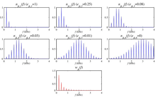
Complex-valued ℓ p norm minimization

ML estimation of the source's STFT coefficients is then converted to ℓp norm minimization ofes(n, f) under the constraint that, e.g. The characterization of the solutions of ℓpnorm minimization for real-valued data also does not hold for complex-valued data [WKSM07].

Time-frequency basis selection

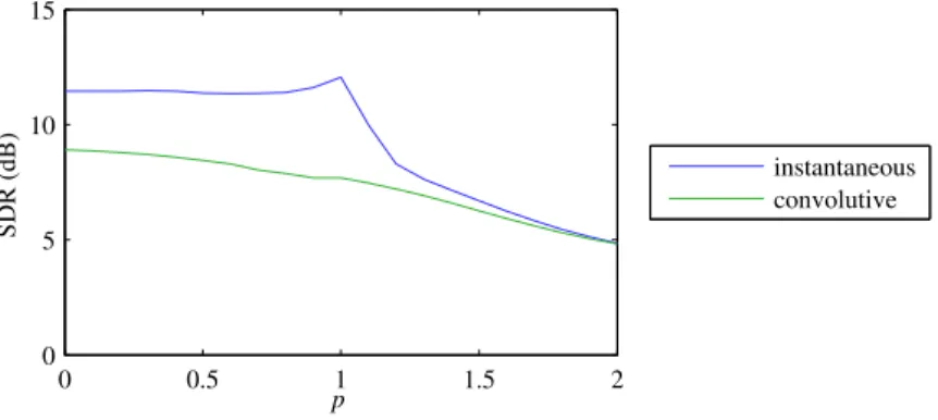
The algorithm with p → 0 ranked first for the separation of instantaneous mixtures in SiSEC 2007 and was later reused as part of the best approximation for underdetermined winding mixtures in SiSEC 2011 [NO12] (see Table 1.2).

Wideband modeling of the mixing filters

Estimation of the source signals

In each iteration, the current estimate is first linearly updated by a combination of the STFT, the iSTFT and filtering according to A(τ) and its adjacency A∗(τ) =A(−τ)T. We also studied the robustness of these algorithms to imprecise estimation of the mixing filters A(τ) by truncation or perturbation with exponentially decaying Gaussian noise [16].

Figure 2.3: Semi-blind separation of a two-channel instantaneous mixture of three speech sources by ℓ p norm minimization with p → 0 [80].

Estimation of the mixing filters

Harmonic sinusoidal modeling of the source signals

Bayesian estimation

I then proposed an efficient algorithm for computing the high-dimensional marginalization integral based on the automatic identification of those variables that are independent a posteriori. I then developed a specific vector quantization technique based on the adaptive interpolation of the amplitudes of the harmonic parts over a set of signal-dependent time and frequency cutoff points.

Greedy estimation

The complex-valued Gaussian distribution is particularly suitable as it results in a closed-form expression for the mixture probability. If the data was generated with a "green" solution dominated by one source, the two channels of the mix are strongly correlated. Once the model parameters are estimated, the STFT coefficients of the source spatial images are derived by multichannel Wiener filteringbcj(n, f) =Wj(n, f)x(n, f)with.

Local Gaussian modeling

ML spatial covariance estimation

The narrowband approximation (2.2) is here equivalent to the assumption that the spatial image channels of the source are perfectly connected to each other and that Σj(f) is a matrix of order 1 equal to toeaj(f)eaj (f)H. For diffuse or echoic sources, the spatial imaging channels of the source are weaker, and we proposed to model Σj(f) as an unbounded full-rank covariance matrix. The parameters vj(n, f) and Σj(f) can be estimated in the ML sense by the following iterative algorithm [15] based on Expectation Maximization (EM) [MK97]: in step E, the zero mean The covariance matrices of the images of estimated resource is calculated as.

Alternative time-frequency representations

Modeling of the spatial covariance matrices

MAP spatial covariance estimation

The expression (3.10) corresponds to a direct-plus-diffuse model, where dj(f) is the anechoic steering vector corresponding to the source DOA, σ2rev is the intensity of echoes and reverberation and Ω(f) is the spatial covariance matrix of a spherically diffuse sound field given by the theory of chamber acoustics [GRT03].

Subspace constraints

Factorization-based modeling of the short-term power spectra

Harmonicity constraints

The spectral jkm(f) is fixed and distributed over a fixed fundamental frequency scale (several possible definitions were investigated in [17]), while only the coefficient sejkms are fitted to the test data, which greatly reduces the dimension of the model. I originally exploited this harmonic NMF algorithm for the task of multiple pitch estimation in polyphonic music signals by using simple thresholding of the activation coefficient shjk(n) to detect the active notes in each time frame [17]. The proposed harmonic NMF algorithm ranked second to the entry of [RK05] in averaging over all data for the note tracking subtask of “Multiple fundamental frequency estimation &.

Figure 3.4: Representation of a basis spectrum with a fundamental frequency of 220 Hz (bottom) as the weighted sum of six narrowband harmonic spectra (top).

Flexible spectral model

Artifact reduction

Bayesian uncertainty estimation

Regarding the initial estimation of the uncertainty around the source signals, a heuristic approach is to assume that the uncertainty in a given time-frequency bin is proportional to the squared difference between the separated sources and the mixture [DNW09, KAHO10]. This bound is iteratively maximized with respect to the auxiliary variables ω and with respect to the parameters of the approximating distributions q(c(n, f))andq(θi)as. 4.8). The results are shown in Figure 4.1 as a function of input signal-to-noise ratio (SNR).

Figure 4.1: Speaker identification accuracy achieved on mixtures of speech and real-world back- back-ground noise with or without source separation, as a function of the input SNR [1].

Uncertainty training

For this particular data and source model, the ML uncertainty estimator (4.1) does not overcome the distortions introduced by source separation and performs worse than the baseline approximation involving no source separation. We reported an improvement of recognition accuracy in the order of 7 to 11% absolute compared to conventional training on clean data and 3 to 4% absolute compared to conventional training on noisy data [6]. More recently, we applied the same approach to singer identification in polyphonic music recordings and achieved a promising accuracy of 94% for 10 classes, compared to 64% without source separation [41].

Evaluation campaigns

We evaluated this algorithm on the same speaker recognition task as above using a different uncertainty propagation technique based on vector Taylor series [MRS96].

Towards multilayer modeling of musical language

Polyphonic pitch and chord modeling

T2 Meter: sequence of measures, each defined by its reference beat and time signature in Vmeter and by the associated metrical accentuation level of each beat and measure subdivision. S5 Instrumentation: beat-synchronized sequence of sets of active voices, each defined by a voice symbol in Vinst (including instruments, band sections, singer identities and sample IDs, with various playing or singing styles). E3 Instrumental timbre: beat-synchronous sequence of vectors of parameters modeling the timbre space of each voice.

Figure 4.2: Draft model of a music piece, from [66]. Dependencies upon overall features are shown in light gray for legibility

Music structure estimation

Note that the problem of joint horizontal and vertical modeling was separately addressed in [MD10] in the context of chord sequences. The above interpolation techniques address all of these issues and we expect them to play an important role in future musical language processing beyond just the problem of polyphonic pitch modeling. In the last eight years since the end of my PhD, audio source separation has become a mature research topic.

Directions

Degrees

Distinctions

Research supervision

Research and technology transfer projects

Collective responsibilities

Signal Processing, Special Issue on Latent Variable Analysis and Signal Separation (2011) Steering committee member, International Conference on Latent Variable Analysis and Signal Separation (LVA/ICA, formerly International Conference on Independent Component Analysis and Signal Separation) (2010) . First French Conference of Young Researchers on Auditing, Musical Acoustics and Audio Signal Processing (JJCAAS) (40 participants, 2003). Founding Chair, CHiME Word Sharing and Recognition Challenge (1 edition with 13 entries in 2011, 2nd edition ongoing).

Keynotes and tutorials

Teaching

Uncertainty-based learning of acoustic models from noisy data. Computer Speech and Language, to appear. Polyphonic pitch estimation and instrument identification by joint modeling of sustained and attack sounds. IEEE Journal of Selected Topics in Signal Processing, vol. Beyond the narrowband approach: Wideband convex methods for underdetermined reverberant sound source separation.

Book chapters

Invited papers in international conferences

Invited papers in national conferences

Peer-reviewed papers in international conferences

Non-negative matrix factorization and spatial covariance model for underdetermined reverberant sound source separation. Underdetermined reverberant sound source separation using local perceived covariance and auditory-motivated time-frequency representation. An experimental evaluation of Wiener filter smoothing techniques applied to underdetermined sound source separation.

Peer-reviewed papers in national conferences

Extended abstracts

Theses

Technical reports

Patents

Software

Data

Séparation de sources

Campagne (SASSEC) [35] que j'ai proposé une méthodologie de référence pour l'évaluation basée sur un ensemble de tâches à résoudre, des critères d'évaluation et des repères de performance. Le problème de séparation de sources se traduit donc par deux tâches différentes selon la nature ponctuelle des sources ou non et selon l'application : l'estimation des signaux sources j(t) ou l'estimation de leur image spatiale cj(t)[10, 35]. Inspiré par les critères définis lors de ma thèse pour l'évaluation des signaux sources [24], j'ai défini un ensemble de critères pour évaluer l'image spatiale estimée bcj(t) d'une source par rapport à une référence de signal cj(t) supposée connue. [10, 35].

Estimation de la structure musicale

Modèles linéaires des signaux audio et algorithmes associés

Principe général
Modélisation parcimonieuse locale
Modélisation à large bande des filtres de mélange
Modélisation sinusoïdale harmonique des signaux sources

J'ai étendu cette approche à la minimisation de la norme ℓp des coefficients TFCT des sources pour p < 2[80]. Cet algorithme a obtenu les meilleures performances sur les mélanges instantanés lors de la campagne d'évaluation SASSEC [35]. Nous avons conçu un algorithme de séparation de sources basé sur ce modèle en minimisant la normeℓ1 des coefficients TFCT des sources grâce à un seuillage itératif doux [16].

Modèles de variance des signaux audio et algorithmes associés

Principe général

MODÈLES DE VARIANCE DU SIGNAL AUDIO ET ALGORITHMES ASSOCIÉS73C.2.4 Modélisation harmonique sinusoïdale des signaux sources.

Modélisation et estimation des matrices de covariance spatiale

Modélisation par factorisation des spectres de puissance à court terme . 74

Description des contenus multi-sources et multi-niveaux

Vers une description robuste des contenus multi-sources

DESCRIPTION DES CONTENUS MULTI-SOURCES ET MULTI-NIVEAUX 75et la régularité des spectres en les factorisant comme la somme des spectres harmoniques. Dans ce cadre existant, nous avons formalisé l'estimateur d'incertitude bayésien exact et conçu un algorithme pratique d'estimation du modèle source [8] basé sur une approche variationnelle bayésienne [1, 39]. Nous avons également montré comment exploiter l'incertitude pour l'apprentissage de classificateurs directement sur des signaux multi-sources et son impact pour des tâches de reconnaissance de locuteurs dans un environnement domestique bruyant [6] ou de reconnaissance de chanteurs dans la musique polyphonique [41].

Vers une modélisation multi-niveaux du langage musical

Conclusion et perspectives

Réalisations

La plupart des techniques actuelles sont basées sur des heuristiques et, dans ce contexte, le cadre bayésien d'estimation de l'incertitude proposé semble prometteur. La modélisation multi-niveaux de la musique reste un problème difficile dont nous n’avons jusqu’à présent qu’effleuré la surface.

Directions

Hybrid approach to multichannel source separation combining time-frequency masking with multichannel Wiener filter. Statistical properties of STFT ratios for two-channel systems and blind source allocation applications. Clustering of separated frequency components by estimating propagation model parameters in blind source separation in the frequency domain.