Volume7, Number2, June2014 pp.X–XX
GAS-SURFACE INTERACTION AND BOUNDARY CONDITIONS FOR THE BOLTZMANN EQUATION
St´ephane Brull, Pierre Charrier and Luc Mieussens
Institut de Math´ematiques de Bordeaux ENSEIRB-MATMECA, IPB
Universit´e de Bordeaux F-33405 Talence cedex, France
(Communicated by Kazuo Aoki)
Abstract. In this paper we revisit the derivation of boundary conditions for the Boltzmann Equation. The interaction between the wall atoms and the gas molecules within a thin surface layer is described by a kinetic equation introduced in [10] and used in [1]. This equation includes a Vlasov term and a linear molecule-phonon collision term and is coupled with the Boltzmann equation describing the evolution of the gas in the bulk flow. Boundary con- ditions are formally derived from this model by using classical tools of kinetic theory such as scaling and systematic asymptotic expansion. In a first step this method is applied to the simplified case of a flat wall. Then it is extented to walls with nanoscale roughness allowing to obtain more complex scattering patterns related to the morphology of the wall. It is proved that the obtained scattering kernels satisfy the classical imposed properties of non-negativeness, normalization and reciprocity introduced by Cercignani [13].
1. Introduction. The Boltzmann equation is a powerful tool to describe phenom- ena in a gas flow taking place at a the scale of the order of the mean free path, i.e.
the micrometric scale (for the air under stantard conditions). For many applications the gas flow takes place in a region bounded by one or several solid bodies. Then boundary conditions have to be prescribed in order to characterize the behavior of the gas close to the wall [13,35].
The first attempt to propose boundary conditions for the Boltzmann equation goes backs to Maxwell in a paper of 1879 ([32]) where he discusses the way to describe the interaction between a gas and a wall. The first condition he proposed corresponds to a simple gas-solid interaction where we assume that the wall is smooth, and perfectly elastic, so that the particles of gas are specularly reflected.
This condition reads
f(t, x, v) =f(t, x, v−2νhν, vi) hv, νi>0, (1) whereν is the unit vector to the surface at pointxandf(t, x, v) is the distribution function of particles that tt time t and position x have the velocity v. Maxwell noticed that this assumption means that the gas can exert any stress on the surface only in the direction of the normal. But this is not physically relevant because in
2010Mathematics Subject Classification. Primary: 82C40, 76P05, 41A60, 82D05; Secondary:
74A25.
Key words and phrases. Kinetic theory, nanoflows, surface diffusion.
1
practical situations it can also exert stress in oblique directions. This is why he introduced another type of boundary conditions corresponding to a more complex gas-solid interaction. Physically he supposed that the wall has a stratum in which fixed elastic spheres are placed. Moreover the stratum is assumed to be deep enough so that every molecule going from the gas to the wall must collide ones or more with the spheres. In this case, the particle is reflected into the gas with a velocity taken with a probability whose density corresponds to the equilibrium state of the gas. In that case the boundary condition (known as the perfect accommodation or diffuse reflexion condition) reads
f(t, x, v) = 1 2π(RT)
Z
hv′,νi<0|hv′, νi|f(t, x, v′)dv′ exp(− v2
2RT), hv, νi>0, (2) whereT is the temperature of the wall. Finally Maxwell considered a more compli- cated intermediate situation which is devoted to be more physically realistic. This model is intermediate between the two previous ones. Maxwell postulated that there is a fraction of the gas which accomdates to the temperature of the solid and another one which is reflected by the solid. In that case the boundary conditions reads
f(t, x, v) = (1−α)f(t, x, v−2νhν, vi)
+ α 1
2π(RT) Z
hv′,νi<0|hv′, νi|f(t, x, v′)dv′ exp(− v2
2RT), hv, νi>0,(3) where T is still the temperature of the wall and α∈[0,1] is called the accomoda- tion coefficient. It represents the tendency of a gas to accomodate to the wall. It means that a fraction of (1−α) of molecules satisfies specular boundary conditions whereas a fraction ofαsatisfies Maxwell diffuse boundary conditions. Whenα= 0, we recover the specular boundary conditions and whenα= 1, we recover the diffuse boundary condition. The main drawback of this condition is that it gives the same accommodation coefficient for energy and momentum though it is known that en- ergy and momentum accommodate differently in physical molecule-wall interactions (see for instance [17]). Nevertheless, this condition has been widely used, both for theoretical studies and numerical simulations for practical applications.
More recently, in [16,13,14,15,18] Cercignani adressed in great details the ques- tion of gas-surface interaction and boundary conditions for the Boltzmann equation with a large bibliography. He introduced a general formulation of the boundary conditions
f(t, x, v)|hν, vi||hν,vi>0= Z
hν,v′i<0
R(v′→v, x, t)f(t, x, v′)|hν, v′i|dv′, (4) where the scattering kernelR(v′ →v, x, t) characterizes the interaction between the molecules of the gas and the molecules of the wall. More preciselyR(v′ →v, x, t) represents the probability density that a molecule stricking the wall with a velocity v′ at pointxand time t is reemitted at the same point with a velocity betweenv andv +dv. To determine the scattering kernel, Cercignani proposed to use either physical or mathematical considerations.
In the physical approach we have to compute as exactly as possible the path of the molecules within the wall. This is anything but easy since such a molecule may experience various events such as elastic scattering, inelastic scattering (including multi-phonon scattering), temporary or permanent adsorption, mobile adsorption (surface diffusion), condensation, reactive interactions. Therefore, in a first attempt,
very simplified models have been used to describe the wall and the interactions such as arrays of smooth hard sphere or hard cubes (see the work of Maxwell and the references given in [15]). A more interesting way to approximate the path of molecules within the wall has been proposed by Cercignani. He suggested to use a transport equation for the molecules inside the solid which is regarded as a half-space. This transport equation includes a Vlasov-type term describing the van der Walls forces exerted on the gas molecules by the solid atoms and a linear collision term (of Boltzmann or Fokker-Plank type) describing the scattering by phonons. Nevertheless, the Maxwell condition (3) can be recovered in this way (with a Boltzmann-like collision term) as well as the Cercignani-Lampis condition [17] (with a Fokker-Plank collision term). This latter condition is free from the physically inconsistence of the Maxwell condition indicated above and has been widely used. More recent works come close to the same approach by determining the molecule-wall interactions by means of molecular dynamics simulation [12,4].
But an intrinsic difficulty in this physical approach is due to our lack of knowledge of the surface layers of solid walls, which leads Cercignani to propose as an alternative that he called the mathematical approach.
The idea of the mathematical approach is to construct a scattering kernel, as simple as possible, satisfying the following basic (physical) requirements:
(i) Non-negativeness:
R(v′→v, x, t)≥0, (5)
(ii) Normalization:
Z
hv,νi>0
R(v′ →v, x, t)dv= 1, (6)
this property means that the mass flux through the boundary vanishes. It is valid when permanent adsorption is excluded.
(iii) Reciprocity:
|hv′, νi|Mw(v′)R(v′ →v, x, t) =|hv, νi|Mw(v)R(−v→ −v′, x, t), (7) whereMwis a Maxwellian distribution having the temperature of the wall. This last property means that the microscopic dynamics is time reversible, and that the wall is in a local equilibrium state and is not influenced by the incoming molecule. An example of a well-known scattering kernel derived in such a way is the Cercignani- Lampis model. We point out that in a recent paper [36], Struchtrup also proposes a new boundary condition that leads to velocity dependent coefficients (as well to isotropic scattering). His approach is close to the mathematical approach as discussed above: velocity dependent accommodation coefficients are introduced into the Maxwell boundary condition, and sufficient conditions are derived so as to ensure properties of normalization and reciprocity. Additional physical arguments lead to coefficients that depend on free parameters that can be adjusted to fit some experimental data.
In the present paper we use the so called physical approach but we start from a somewhat more sophisticated model introduced in [10] and used in [11,7, 8, 9, 30,31,1] for studying gas-surface interaction, nanoflows and surface diffusion. This model, valid for smooth walls, is still a crude approximation of the complex gas surface interaction, but it proved to be remarkably useful to give new insight on these issues. It couples the Boltzmann equation in the bulk flow with a kinetic model inside a very thin surface layer (with width typically less than a nanometer)
where the van der Waals forces are taken into account. This model includes a Vlasov term to take into account the part of the interaction potential that depends on the frozen position of the atoms of the solid wall (the long range interactions), and a Boltzmann like linear collision term between molecules and phonons to take into account the thermal fluctuations of the atoms of the solid (short range interactions).
It contains several characteristic times: the characteristic time of the Boltzmann equation in the bulk flow, the characteristic time of the kinetic model in the surface layer, the characteristic time of flight of a molecule through the surface layer, the characteristic molecule-phonon relaxation time. Then using classical tools of kinetic theory such as scaling asymptotic analysis we can derive various models correspond- ing to different regimes according to the relative value of the characteristic times.
Thus in [1] surface kinetic and surface diffusion models have been derived from this three phase model: they describe mobile adsorption and can be interpreted asnon localboundary conditions. In the present paper, using different scalings, we derive local boundary conditions from the same basic three phase model. First, a weak molecule-phonon interaction regime is considered. In that case the particles of the gas quickly cross the surface layer and the classical specular boundary condition is obtained. Then a strong molecule-phonon interaction is investigated. In this situ- ation the particles of the gas slowly cross the surface layer and are thermalized by the wall leading to Maxwell-diffuse boundary conditions. Finally, an intermediate interaction is assumed, and we get a Maxwell-like boundary condition (3), but with a fraction of diffusely evaporated molecules that depends on the velocity. Moreover, the relationship between this coefficient and the surface-molecule interaction poten- tial is formulated. One of the interesting asset of this boundary condition is that it gives different accommodation coefficients for energy and (normal and tangential) momentum, contrary to the original Maxwell condition. Moreover it must be noted that mobile adsorption (see [1]) as well as elastic or inelastic scattering are treated within the same framework. Finally this analysis is extended to a non-smooth wall with nanoscale roughness assumed to be periodic in the directions parallel to the surface. This leads to a scattering kernel with more complex reflexion patterns that depend on the wall morphology.
This paper is organized as follows. Section 2 deals with the presentation of nanoscale kinetic models describing the interaction between a wall and particles in a very simplifed configuration with a flat wall and simplified expression of the potential. In section 3, the boundary conditions are derived under these assumptions by using asymptotic analysis. In section4, the same analysis is extended to the more realistic case of a wall with nanoscale roughness and a general potential. Section5 is devoted to some comments on these results and to concluding remarks.
2. Nanoscale kinetic models for gas-surface interaction. In this section we recall the nanoscale models describing a gas flow near a wall introduced in [10] and [1]. In these models the interaction between the wall and the gas molecules through Van der Walls forces are taken into account in a thinsurface layer(with thickness L typically smaller than one nanometer). In all the following, for the sake of sim- plicity, we assume that the molecules move in a 2D half-plane 1 and we consider the following configuration: the solid is occupying the half-space z > L, the gas
1As indicated in [1] we can assume that the molecules move in the 3D half-space (x, y, z), z <0, provided thatf is interpreted as the marginal distribution function obtained by integrating the original distribution function with respect tovy.
phase is constituted by the gas molecules in the half-space z < 0, outside of the range of the surface forces, and we consider separately thesurface layer 0< z < L, where the gas molecules move within the range of the surface potential. The gas flow in this surface layer is modelled by the collisionless Boltzmann equation (the size of this layer is much smaller than the mean free path of the molecules), with a Vlasov term to take into account the part of the interaction potential that depends on the frozen position of the atoms of the solid wall (the long range interactions), and a collision term between molecules and phonons to take into account the ther- mal fluctuations of the atoms of the solid (short range interactions) (see [10] for a physical justification of this approach). Since in many applications the surface potential is an attractive-repulsive potential, some of the molecules in the surface layer have a total energy which is too small to escape from the potential well and aretrappedin the surface layer. On the other hand some molecules, called the free molecules, have enough energy to escape from the potential well and can leave the surface layer and go into the bulk flow.
Both type of molecules (trapped and free) are taken into account in this approach and we give now more details on the model describing their motion in the surface layer.
2.1. The surface potential. We assume that the wall is flat and we use a simpli- fied interaction potential which reads
V(x, z) =W(z), (8)
whereW is an attractive-repulsive potential, ie;
(H1) 0≤W(z) ,
(H2) limz→LW(z) = +∞,
(H3) the potentialW is repulsive (i.e. W′(z)>0) forzm≤z < Land is attractive (W′(z)<0) for 0< z < zm, and we setW(zm) = 0
(H4) The range of the surface forces is finite and thus, the potential satisfiesW(z) = Wmforz <0.
This simplified potential allows to uncouple the parallel motion and the normal motion of gas molecules near the solid wall, which makes the mathematical devel- opments much easier. Moreover, though not physically realistic, this potential is sufficient to obtain accurate information on the behavior of the gas near the walls (see [1] for more details). Extension to a more realistic interaction potential is considered in section4.
It is useful to introduce in the surface layer the following velocity variable, called equivalent velocity:
ez=sign(vz)p
v2z+ 2W(z)/m, (9)
which is the velocity of a particle whose total energy12mvz2+W(z) would be a kinetic energy 12me2z only. We denote by e= (vx, ez) the corresponding two dimensional velocity.
It will be more convenient to describe the distribution function of gas molecules in the surface layer as a function oferather than a function of (vx, vz).
Now, we explain how particles can be divided into two different classes: the free particles and the trapped particles. The trajectory of a particle along z is defined (if there is no collision) by the two differential equations z′(t) = vz(t)
and mv′z(t) =∂zW(z(t)). Along this trajectory, the total energy 12mv2z+W(z) is constant. According to the definition of the equivalent velocityez(see (9)), we have
1
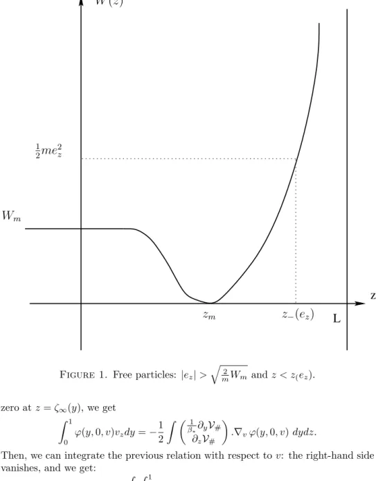
2me2z=12mvz2+W(z) which is a constant too. A particle is free if it can leave the surface layer and go into the gas. In this case, the potential reaches the valueWm, and since its kinetic energy 12mv2z is non-negative, this means that 12me2z > Wm, which is equivalent to|ez|>q
2
mWm. The limit position of this particle when it is inside the surface layer is such that it takes a zero velocity. At this point, denoted byz−(ez), we haveW(z−(e(z))) = 12me2z (see figure1).
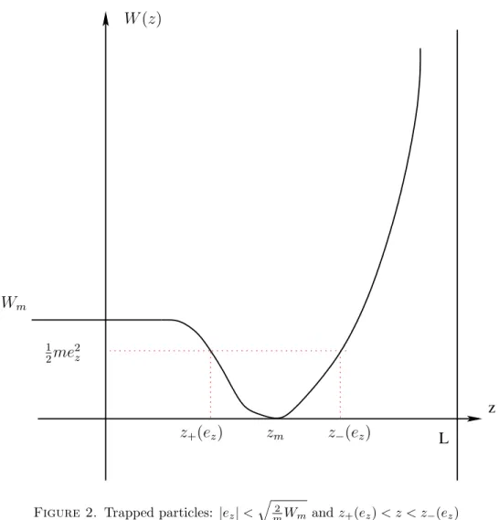
At the contrary, a particle is trapped if its total energy is lower thatWm, that is to say|ez| <q
2
mWm. In that case, the potential is bounded by 12me2z < Wm, which means that z varies between two limit values z+(ez) and z−(ez) such that W(z±(ez)) = 12me2z(see figure2): the particle cannot escape from the surface layer.
In order to have the same notation for trapped and free particles, we setz+(ez) = 0 for free particles (that is to say, if|ez|>q
2
mWm). Moreover, for particles with zero total energy, we haveez= 0 and hence the velocity and the potential are zero too, which means that the particle stay at positionz=zm. The we setz±(0) =zm
in this case.
With this definition, note thatz+ andz− are even functions ofez.
Now, we introduce some notations that are useful to switch between vz andez
variables. The velocity of a particle with equivalent velocityez located at position z∈[z+(ez), z−(ez)] is given by
vz(z, ez) =sign(ez) r
e2z− 2
mW(z), (10)
and we have
vz(z−(ez), ez) =vz(z−(−ez),−ez) = 0. (11) Moreover, for trapped molecules we also have
vz(z+(ez), ez) =vz(z+(−ez),−ez) = 0. (12) Let us define
σ(z, ez) = 1
|vz(z, ez)| = (e2z− 2
mW(z))−1/2 for|ez|>p
2W(z)/m, so that
σ(z, ez)vz(z, ez) =sign(ez), (13) and also
τz(ez) =
Z z−(ez)
z+(ez)
σ(z, ez)dz=
Z z−(ez)
z+(ez)
(e2z− 2
mW(z))−1/2dz.
As in [24], τz(ez) can be interpreted as the time for a molecule to cross the surface layer. Moreover, for everyz∈]0, L] the applicationvz→ezis a one-to-one applica- tion from [0,+∞[ onto [q
2
mW(z),+∞[ and from ]− ∞,0] onto ]− ∞,−q
2 mW(z)].
Therefore differentiating (10) leads to
dvz=|ez|σ(z, ez)dez. (14)
Thus the integral of a given function ψ(z, vz) with respect to vz can be trans- formed as follows:
Z
vz
ψ(z, vz)dvz= Z
|ez|>√2
mW(z)
ψ(z, vz(z, ez))|ez|σ(z, ez)dez. (15) Moreover, the order of integration in az-ezintegral can be changed as follows (see figure3):
Z L
0
Z
|ez|>√2 mW(z)
ψ(z, vz(z, ez))|ez|σz(z, ez)dez
! dz
= Z +∞
−∞
Z z−(ez)
z+(ez)
(ψ(z, vz(z, ez))|ez|σ(z, ez)dz
! dez.
(16)
2.2. Molecule-phonon collision term. In this paper we consider the general molecule-phonon collision term
Q[φ](v) = Z
IR2
K(v, v′) exp
−m|v|2 2kT
φ(v′)−exp
−m|v′|2 2kT
φ(v) dv′. With the new velocity variable e = (vx, ez) defined in (9), for a given value ofz, this operator reads:
Q[φ](z, e) =Q+[φ](z, e)−Q−[φ](z, e) = Z
E(z)
K(z, e, e′) (G(e)φ(e′)
−G(e′)φ(e))Je′ de′,
(17) whereE(z) ={e′, |e′z| ≥p
2W(z)/m}, Je′ =J(z, e′z) =|e′z|σ(z, e′z), and G(e) = exp
−m(|vx|2+|ez|2) 2kT
. (18)
The collision kernelKis such that k(z, e→e′) =K(z, e, e′)G(e′) is the probability of transition per unit time from the state eto the state e′ in a “collision” with a phonon. The dimension of K is [time/length2] (or, if the molecules move in a 3D plane, of [time2/length3]). We assume in the following that
K(z, e, e′) = K(z, e′, e),
0< ν0 ≤ K(z, e, e′)≤ν1, (19) K(z, vx,−ez, vx′,−e′z) = K(z, vx, ez, vx′, e′z), (20)
K(z,−vx, ez, v′x, e′z) = K(z, vx, ez, vx′, e′z).
The loss term of the molecule-phonon collision term can be written Q−[φ](z, e) = 1
τms(z, e)φ(z, e), (21)
where
τms(z, e) = Z
E(z)
K(z, e, e′)G(e′)J(z, e′z)de′
!−1
(22) is a collision time (at pointz). It is useful for the sequel to introduce the mean relax- ation timeτms(e) defined as the harmonic mean ofτms(z, e) weighted byσ(z, ez):
1 τms(e) =
Rz−(ez)
0 σ(z, ez)/τms(z, e)dz Rz−(ez)
0 σ(z, ez)dz =
Rz−(ez)
0 σ(z, ez)/τms(z, e)dz
τz(ez) . (23)
Using (20), the even parity ofσ,G,J andz±with respect toez, and the symmetry ofE(z), we have :
τms(z, vx,−ez) =τms(z, vx, ez), and τms(vx,−ez) =τms(vx, ez).
Let us remark that if we assumeK(z, e, e′) = 1, thenτm does not depends one and we have:
Q[φ] = 1 τms(z)
n[φ]
γ(z)G−φ
, (24)
where γ(z) = τms(z)−1 = R
E(z)G(e′)J(z, e′z)de′ and n[φ] = R
E(z)φ(e′)J(z, e′z)de′, which is quite similar to the BGK-like relaxation term used in [1]. Finally we recall some of the main properties satisfied by the operatorQ.
Proposition 1. The collision term satisfies the following properties Z
E(z)
Q[φ](e)Je de = 0, (mass conservation), (25)
Q[φ] = 0 ⇔ φ=n G, (equilibrium), (26)
Z
E(z)
Q[φ](e)φ(e) Je
G(e)de ≤ −ν0γ(z) Z
E(z)
w2Je
Gde, (H theorem), (27) Z
E(z)
Q[φ](e)ψ(e) Je
G(e)de = Z
E(z)
Q[ψ](e)φ(e) Je
G(e)de, (symmetry) , (28) where we used the macro-micro decomposition φ=q+wwith q=n[φ]Gand where w=φ−q satisfiesn[w] = 0.
2.3. Nanoscale models. The first model introduced in [10] and [1] is the following system of coupled kinetic equations which describes the flow of molecules in the surface layer (where the Van der Waals forces are acting) and outside:
∂tf+vx∂xf+vz∂zf = 0, z <0 (29) f(t, x,0, vx, vz)|vz<0 = φ(t, x,0, vx, ez(0, vz)), (30)
∂tφ+vx∂xφ+vz(z, ez)∂zφ = Q[φ], z+(ez)< z < z−(ez), (31) φ(t, x,0, vx, ez)e
z>√
2Wm/m = f(t, x,0, vx, vz(0, ez)), (32) φ(t, x, z−(ez), vx, ez) = φ(t, z−(−ez), vx,−ez), (33) φ(t, x, z+(ez), vx, ez) = φ(t, z+(−ez), vx,−ez), |ez|<p
2Wm/m,(34) wheref =f(t, x, z, vx, vz) is the distribution function describing the bulk flow and φ= φ(t, x, z, vx, ez) is the distribution function describing the gas flow inside the surface layer. Let us remark that since we have chosen to define φas a function of (vx, ez) equation (31) does not contain a Vlasov term in the z-direction.
The above model describes the gas-solid interaction at the nanoscale, i.e on a domain [0, x∗]×[−z∗, L] withx∗ andz∗ ≈ 1 nanometer. But on a larger scale in the tangential direction, this model is too complicated and contains stiff terms that would make its numerical solution too much expensive. Thus in [1] the authors derived a limit model obtained by asymptotic analysis when the domain is much larger than the surface layer (that is to sayx⋆ ≈z∗≫L). In this model, the flow of molecules in the surface layer is described by a one-dimensional kinetic equa- tion which can be considered as a nonlocal boundary condition for the Boltzmann equation in the bulk flow.
But on a larger scale inxandzthis last model is still too complicated to manage and it would be interesting to investigate the relation between these nanoscale models and the standard boundary conditions used with the Boltzmann equation in gas kinetic theory.
In the following, we use the nanoscale model (29-34) to derive various boundary conditions for the Boltzmann equation (29), according to convenient scalings.
3. Derivation of boundary conditions: Case of a flat wall. In this section, we assume that the characteristic times of the flow in the surface layer (the time for a molecule to cross the surface layer and the relaxation time of molecules by phonons) are much smaller than the characteristic time of evolution of the bulk flow.
We derive boundary conditions for the Boltzmann equation in the bulk flow by an asymptotic analysis of system (29-34). The main point in this derivation is to find the solution of a linear kinetic problem which describes, in a first approximation, the motion of the molecules in the surface layer. Unfortunately this problem cannot be solved exactly but approximated solutions can be obtained (see Lemma 1 after the proof of Proposition2).
We consider system (29-34) and we introduce the following dimensionless quan- tities:
˜ n= n
n∗,˜vx=vx
v∗,v˜z =vz
v∗,e˜z= ez
v∗,f˜= f
f∗,φ˜= φ
f∗,˜x= x l∗, W˜ = W
W∗,W˜m= Wm
W∗,˜t= t
t∗B,τ˜z = τz
τz∗,˜τms= τms
τms∗ ,K˜ = K K∗,
and ˜z = lz∗ for the Boltzmann equation in the bulk flow, while ˜z = Lz in the surface layer. The reference quantities are the followings:n∗is the reference number density, v∗ =p
kT /m, f∗ =n∗/v∗2, t∗B is the reference time of evolution for the Boltzmann equation (29), l∗ = v∗t∗B, τms∗ = 1/(K∗v∗2) is a reference relaxation time,τz∗=L/v∗is the characteristic time of flight of a molecule through the surface layer, andW∗=mv∗2/2.
In order to study different regimes corresponding to different order of magni- tude of the characteristic time scales τz∗, τms∗ and t∗B, we introduce the following nondimensional parameters:
ε=τms∗
t∗B and η= τms∗ τz∗ . Then system (29-34) reads in dimensionless form
∂˜tf˜+ ˜vx∂˜xf˜+ ˜vz∂˜zf˜ = 0, z <˜ 0, (35) f˜(˜t,x,˜ 0,˜vx,v˜z)v˜z<0 = φ(˜˜ t,x,˜ 0,v˜x,e˜z(0,v˜z)), (36)
∂˜tφ˜+ ˜vx∂˜xφ˜+η
ε˜vz(˜z,e˜z)∂z˜φ˜ = 1
εQ[ ˜˜ φ], z˜+(˜ez)<z <˜ z˜−(˜ez), (37) φ(˜˜ t,x,˜ 0,v˜x,˜ez)v˜z>0 = f˜(˜t,x,˜ 0,v˜x,v˜z(0,e˜z)), (38) φ(˜˜ t,x,˜ z˜−(˜ez),v˜x,˜ez) = φ(˜˜ t,z˜−(˜ez),˜vx,−˜ez), (39) φ(˜˜ t,x,˜ z˜+(˜ez),v˜x,˜ez) = φ(˜˜ t,z˜+(˜ez),˜vx,−˜ez), for|e˜z|<
qW˜m.(40) We mention that with this dimensionless variables, a particle of velocityezlocated atz is:
• either trapped if |e˜z˜| < pW˜m, and hence stays between ˜z±(˜ez˜) defined by W˜(˜z±(˜ez)) = ˜e2z,
• or free if|˜ez|>pW˜m, and hence stays on the left-hand-side of ˜z−(˜ez) defined by ˜W(˜z−(˜ez)) = ˜e2z. We set ˜z+(˜ez˜) = 0 in this case.
We can obtain boundary conditions for the Boltzmann equation through an as- ymptotic analysis of the above system when ε → 0. This leads to the following results.
Proposition 2. Under the hypothesis (8) and (H1-H4), in the limit ε → 0, the gas-surface interaction depends on the order of magnitude ofη and can be described by the following boundary conditions atz= 0:
1. for η=O(1ε), the boundary condition is the specular reflection f(t, x,0, vx, vz)|vz<0 = f(t, x,0, vx,−vz).
2. for η =O(ε), the boundary condition is the reflection with perfect accommo- dation
f(t, x,0, vx, vz)|vz<0 = κ(t, x)M(vx, vz), (41) where
κ(t, x) = Z
vz>0
Z
vzf(t, x,0, vx, vz)dvxdvz/ Z
vz>0
Z
vzM(vx, vz)dvxdvz
is such that the mass flux of f through the boundaryz= 0is zero, and where M(v) = exp −m(vx2+vz2)/2kT
.
3. for η =O(1), the boundary condition can be approximated by a Maxwell-like boundary condition
f(t, x,0, vx, vz)|vz<0=a(v)β(t, x)M(v) + (1−a(v))f(t, x,0, vx,−vz), where
a(v) = 1−exp
−2ˆτz(vz) ˆ τms(v)
, (42)
β(t, x) = Z
vz>0
Z
vza(v)f(t, x,0, vx, vz)dvxdvz/ Z
vz>0
Z
vza(v)M(vx, vz)dvxdvz, with the notationsˆτz(vz) =τz(ez(0, vz))andτˆms(v) =τms(vx, ez(0, vz)). This boundary condition ensures a zero mass flux of f at the boundary z = 0.
Moreover, it can be written under the general form (4) with a scattering kernel R(v′→v)that satisfies the properties of non-negativeness, normalization and reciprocity.
Proof. In order to simplify the notations, the tilde˜over the dimensionless quantities are dropped in the following. To avoid confusion, we will indicate explicitely when we come back to dimensional quantities.
In order to perform an asymptotic analysis of system (35-40), we look for a solution in the form
f =fε=f0+εf1+..., φ=φε=φ0+εφ1+....
This expansion is inserted into (35–40) and we identify the terms of same power of magnitude w.r.tε.The zeroth-order termf0 satisfies
∂tf0+vx∂xf0+vz∂zf0 = 0, (43)
f0(t, x,0, vx, vz)vz<0 = φ0(t, x,0, vx, ez(0, vz)). (44)
However, the zeroth-order termφ0 depends on the order of magnitude of η.
(1) We consider the caseη =O(1ε). This means that τz∗≪τms∗ ≪t∗B,
that is to say the free time of flight of a molecule to cross the surface layer is much smaller than the relaxation time of molecules by phonons. Thus the flow of molecules crosses the surface layer so quickly that the relaxation phenomena can be neglected. Then φ0 satisfies the following linear kinetic surface layer (LKSL) problem:
vz(z, ez)∂zφ0 = 0, forz+(ez)< z < z−(ez), (45) φ0(t, x,0, vx, ez)ez>√Wm = f0(t, x,0, vx, vz(0, ez)), (46) φ0(t, x, z−(ez), vx, ez) = φ0(t, x, z−(ez), vx,−ez), (47) φ0(t, x, z+(ez), vx, ez) = φ0(t, x, z+(ez), vx,−ez), for|ez|<p
Wm. (48) Consider some vz < 0 and the boundary condition (44) where we write ¯ez = ez(0, vz):
f0(t, x,0, vx, vz)vz<0=φ0(t, x,0, vx,e¯z). (49) Since (45) implies that φ0 does not depend on z, we can replace z = 0 in the right-hand side of (49) by z=z−(ez) to get
f0(t, x,0, vx, vz)vz<0=φ0(t, x, z−(¯ez), vx,e¯z).
Moreover (47) and the even parity ofz− imply
f0(t, x,0, vx, vz)vz<0=φ0(t, x, z−(−e¯z), vx,−¯ez).
Again, we use the fact thatφ0 does not depend onzto get f0(t, x,0, vx, vz)vz<0=φ0(t, x,0, vx,−e¯z), where, by definition,−e¯z≥√
Wm. Now we can use (46) to replace the right-hand side of the previous relation and to get the specular boundary condition
f0(t, x,0, vx, vz)vz<0 = f0(t, x,0, vx,−vz).
We mention that we used η = O(1ε) for simplicity. In fact, we recover the same boundary condition ifη=O(ε−α), for every positiveα.
(2) Now we assumeη=O(ε), which implies that τms∗ ≪τz∗ ≪t∗B.
This means that the relaxation time of molecules by phonons is much smaller than the free time of flight of a molecule to cross the surface layer. In this limit the flow of incoming molecules into the surface layer immediately relaxes toward the equilibrium. Now the LKSL problem satisfied byφ0 reads
Q[φ0] = 0, forz+(ez)< z < z−(ez), (50) φ0(t, x,0, vx, ez)ez>0 = f0(t, x,0, vx, vz(0, ez)), (51) φ0(t, x, z−(ez), vx, ez) = φ0(t, z−(ez), vx,−ez), (52) φ0(t, x, z+(ez), vx, ez) = φ0(t, x, z+(ez), vx,−ez), for|ez|<p
Wm (53) which gives
φ0(t, x, z, vx, ez) =α(t, x)G(vx, ez), forz+(ez)< z < z−(ez). (54)
However, the distribution function φ0 is Maxwellian and hence cannot satisfy the inflow boundary condition (51). Thus we have to introduce in the expansion ofφa Knudsen-layer corrector
φ(t, x, z, vx, ez) =φ0(t, x, z, vx, ez) +ψ0(t, x,z
ε, vx, ez) +εφ1(t, x, z, vx, ez) +..., where φ0 is still defined by (54) and satisfies (50, 52, 53), and ψ0(t, x, y, vx, ez) is given by
vz(0, ez)∂yψ0 = Q0[ψ0], for|ez| ≥p
Wm, 0< y <+∞, (55) ψ0(t, x,0, vx, ez)|ez>0 = f0(t, x,0, vx, vz(0, ez))−φ0(t, x,0, vx, ez), (56) and should rapidly decrease to 0 for largey. Note thatQ0is defined by
Q0[χ] = Z
E(0)
K(0, e, e′) (G(e)χ(e′)−G(e′)χ(e))J(0, e′)de′. Then, it is useful to introduceχ(t, x, y, vx, ez) defined by
χ(t, x, y, vx, ez) =ψ0(t, x, y, vx, ez) +φ0(t, x,0, vx, ez), (57) which implies thatχis the unique bounded solution of the following linear half-space problem
vz(0, ez)∂yχ = Q0[χ] (58)
χ(t, x,0, vx, ez)|ez>0 = f0(t, x,0, vx, vz(0, ez)). (59) A standard assumption gives the following outgoing distribution (it was for instance used in [23] to compute extrapolation length, see also [26]), which is often sufficient in many kinetic boundary layer computations:
χ(t, x, y, vx, ez)|ez<0≈χ(1)(t, x, y, vx, ez)|ez<0=κ(t, x)G (60) for every y ≥ 0, where κ can be determined as follows. Another standard re- sult on the linear half-space problem (58–59) shows that χ necessarily satisfies R
E(z)ezχ(t, x, y, vx, ez)de = 0 for every y (see, for instance [19, 21, 33]). Then, writing this relation at y = 0 and using the boundary condition (59) and the ap- proximation (60) give the definition
κ(t, x) =− R
ez>0 inE(0)ezf0(t, x,0, vx, vz(0, ez))de R
ez<0 inE(0)ezG(e)de
= R
vz>0
Rvzf0(t, x,0, vx, vz)dvxdvz
R
vz>0
R vzM(vx, vz)dvxdvz
,
(61)
whereM(vx, vz) =G(vx, ez(0, vz)) = exp(−(vx2+vz2)/2).
Now, note that (44) has to be modified according to the Knudsen layer correction to get
f0(t, x,0, vx, vz)vz<0=φ0(t, x,0, vx, ez(0, vz)) +ψ0(t, x,0, vx, ez(0, vz))
=χ(t, x,0, vx, ez(0, vz)).
Consequently, the definition (57) ofχand the approximation (60) give the following approximation of the outgoing distribution
f0(t, x,0, vx, vz)vz<0≈κ(t, x)M(vx, vz), (62)
which gives in dimensional variables the classical perfect accommodation boundary condition (41) (sometimes called the diffuse reflexion boundary condition), provided that the coefficientκis such that the corresponding approximation of the mass flux of f0 at the boundaryz = 0 is zero. Indeed, the definition (61) of κimplies that this property holds.
(3) Finally, we assume η =O(1), which corresponds to τms∗ ≈ τz∗ ≪ t∗B. The LKSL problem satisfied byφ0 is
vz(z, ez)∂zφ0 = Q[φ0], forz+(ez)< z < z−(ez), (63) φ0(t, x,0, vx, ez)ez>√Wm = f0(t, x,0, vx, vz(0, ez)), (64) φ0(t, x, z−(ez), vx, ez) = φ0(t, x, z−(ez), vx,−ez), (65) φ0(t, x, z+(ez), vx, ez) = φ0(t, x, z+(ez), vx,−ez), for|ez|<p
Wm. (66) We can claim that this linear kinetic surface layer (LKSL) problem has a unique solution and that this solution has a zero mass flux through the surfacez= 0 (see Lemma3.1after this proof):
Z
|ez|>√ Wm
Z
ezφ0(t, x,0, vx, ez)dvxdez= 0. (67) Now if we solve the LKSL problem (63-66), then φ0(t, x,0, vx, ez), which is the value of the solution at z = 0 for ez <0, gives a boundary value for (44). This value linearily depends on the inflow data: φ0(t, x,0, vx, ez(0, vz)) =A(f0(t, x,0, vx, .)|vz>0), whereAis called the “albedo” operatorA. Consequently, the boundary condition (44) of (43) reads
f0(t, x,0, vx, vz <0) =A(f0(t, x,0, vx, .)|vz>0). (68) This relation can be interpreted as an exact boundary condition. However, the operatorAis implicitely defined: we must solve the LKSL problem (63-66) to get φ0(t, x,0, vx, ez)ez<0, which could be done approximately by a numerical computa- tion. Nevertheless, it is possible to get an approximation of the operator A that explicitely gives φ0(t, x,0, vx, ez)ez<0 as a function of f0(t, x,0, vx, vz(0, ez))|ez>0: using again Lemma3.1(see after this proof), we can conclude that
φ0(t, x,0, vx, ez)ez<0 = (1−a(ez))f0(t, x,0, vx,−vz(0, ez)) +a(ez)α(t, x)G(vx, ez).
From (44), we get
f0(t, x,0, vx, vz)vz<0 = φ0(t, x,0, vx, ez(0, vz))
= (1−a(vz))f0(t, x,0, vx,−vz) +a(vz)β(t, x)M(vx, vz).
Moreover, for the same reason as for the previous regime, the approximation of the mass flux of f0 through the boundary z = 0, and hence the coefficient β can be uniquely determined. Coming back in dimensional variables, we get (3). From this relation we can easily check that the associated scattering kernel satisfies the properties of non-negativeness, normalization and sincea(v) =a(−v), the property
of reciprocity.
Lemma 3.1. Let us consider the linear kinetic surface layer problem (LKSL) vz(z, ez)∂zφ0 = Q[φ0], for z+(ez)< z < z−(ez), (69) φ0(0, vx, ez)ez>√Wm = f∗(vx, vz(0, ez)), (70) φ0(z−(ez), vx, ez) = φ0(z−(ez), vx,−ez), (71) φ0(z+(ez), vx, ez) = φ0(z+(ez), vx,−ez), for|ez|<p
Wm. (72) This problem has a unique solution and this solution has a zero mass flux through the surface z= 0:
Z
|ez|>√ Wm
Z
ezφ0(0, vx, ez)dvxdez= 0, (73) and we have
φ0(0, vx, ez)|ez<−√Wm = (1−a(e))f∗(vx,−vz(0, ez)) +h∗[φ0](e)G(e), (74) where the coefficientais given by
a(e) = 1−exp
−2τz(ez)
¯ τms(e)
. (75)
Moreover, if we assume that Q+(φ0) =Q+(αG), whereα depends on f∗ but does not depend onz,vx, andez, then we have
φ0(0, vx, ez)|ez<−√Wm = (1−a(e))f∗(vx,−vz(0, ez)) +a(e)α1G(vx, ez), (76) andαis determined by (73) (see (84) in the proof ).
Proof. (i) Existence and uniqueness. Existence and uniqueness of a solution of the LKSL problem (69-72) can be proved by using standard techniques in linear transport problems. The reader can refer, for instance, to [25].
(ii) Mass flux at z= 0. Multiplying (69) by|ez|σ(z, ez) and using (13), we get ez∂zφ0=Q[φ0]|ez|σ(z, ez).
Now we integrate this relation with respect toz. It comes Z z−(ez)
z+(ez)
ez∂zφ0dz=
Z z−(ez)
z+(ez)
Q[φ0]|ez|σ(z, ez)dz, or,
ezφ0(z−(ez), vx, ez)−ezφ0(z+(ez), vx, ez) =
Z z−(ez)
z+(ez)
Q[φ0]|ez|σ(z, ez)dz, wherez+(ez) = 0 for |ez|>√
Wm. Now integrating with respect tovx and ez, we find
Z Z
ezφ0(z−(ez), vx, ez)dvxdez− Z Z
ezφ0(z+(ez), vx, ez)dvxdez
=
Z Z Z z−(ez)
z+(ez)
Q[φ0]|ez|σ(z, ez)dzdvxdez. (77)
But sinceezφ0(z±(ez), vx, ez)dvxdez is an odd function of ez (see (71) and (72)), the first term of the left-hand side of this relation vanishes and the second one gives
Z Z
ezφ0(z+(ez), vx, ez)dvxdez = Z Z
|ez|<√ Wm
ezφ0(z+(ez), vx, ez)dezdvx
+ Z Z
|ez|>√ Wm
ezφ0(0, vx, ez)dezdvx,
= Z Z
|ez|>√ Wm
ezφ0(0, vx, ez)dezdvx. Consequently, (77) now reads
− Z Z
|ez|>√ Wm
ezφ0(0, vx, ez)dezdvx=
Z Z Z z−(ez)
z+(ez)
Q[φ0]|ez|σ(z, ez)dzdvxdez. Finally, inverting the integration with respect tozand the integration with respect tovx andez in the right-hand side (see (16)), we get
− Z Z
|ez|>√ Wm
ezφ0(0, vx, ez)dvxdez = Z L
0
Z
E(z)
Q[φ0]|ez|σ(z, ez)dedz,
= 0, due to the mass conservation (see (25)).
(iii) Approximate solution of the LKSL problem. As indicated in the proof of proposition2(point 3), the LKSL problem (69–72) has a unique solutionφ0, and the relation
φ0|e
z<−√
Wm =A[φ0|e
z>√
Wm] (78)
leads to a boundary condition for the Boltzmann equation which is, unfortunately, implicit. We are going to show how we can obtain an explicit relation between φ0
|ez<−√
Wm andφ0
|ez>√
Wm which can be considered as an approximation of (78).
In a first step we give a more explicit expression of the albedo operatorA. We first note that
Q+[φ0] = Z
E(z)
K(z, e, e′)φ0(e′)Je′de′
! G(e)
= b[φ0](z, e)G(e). (79)
Moreover, we multiply (69) byσ(z, ez) and we use (79) to rewrite (69) as sign(ez)∂zφ0=σ(z, ez)Q+[φ0]− σ(z, ez)
τms(z, e)φ0, forz+(ez)< z < z−(ez). (80) Then, we integrate (80) along trajectories. Since (78) defines the distribution of outgoing particles, that are all free particles, we shall make this integration for|ez|>
√Wmonly (see at the end of this proof for a remark about trapped particles). First, particles with positiveez go fromz+(ez) = 0 to z−(ez), and we can integrate (80)