[PENDING] Equilibres de Nash dans les jeux concurrents : application aux jeux temporisés

(1)

HAL Id: tel-00827027

https://tel.archives-ouvertes.fr/tel-00827027

Submitted on 28 May 2013

HAL is a multi-disciplinary open access archive for the deposit and dissemination of sci- entific research documents, whether they are published or not. The documents may come from

L’archive ouverte pluridisciplinaire HAL, est destinée au dépôt et à la diffusion de documents scientifiques de niveau recherche, publiés ou non, émanant des établissements d’enseignement et de

Equilibres de Nash dans les jeux concurrents : application aux jeux temporisés

Romain Brenguier

To cite this version:

Romain Brenguier. Equilibres de Nash dans les jeux concurrents : application aux jeux tempo- risés. Autre [cs.OH]. École normale supérieure de Cachan - ENS Cachan, 2012. Français. �NNT : 2012DENS0069�. �tel-00827027�

(2)

ENSC-201X-N^oYYY

TH`ESE DE DOCTORAT

DE L’´ECOLE NORMALE SUP´ERIEURE DE CACHAN

Pr´esent´ee par Monsieur Romain Brenguier

Pour obtenir le grade de

DOCTEUR DE L’´ECOLE NORMALE SUP´ERIEURE DE CACHAN

Domaine : Informatique

Titre :

Equilibres de Nash dans les Jeux Concurrents´ – Application aux Jeux Temporis´es Nash Equilibria in Concurrent Games

– Application to Timed Games

Thèse présentée et soutenue à Cachan le 29 novembre 2012 devant le jury com- posé de :

Christof L¨oding Rapporteur

Anca Muscholl Rapporteur

Hugo Gimbert Rapporteur

Kim G. Larsen Examinateur

Jean-Fran¸cois Raskin Examinateur

Patricia Bouyer-Decitre Directrice de th`ese

Nicolas Markey Directeur de th`ese

Laboratoire Spécification et Vérification ENS Cachan, CNRS, UMR 8643 61, avenue du Président Wilson 94235 CACHAN Cedex, France

(3)

(4)

Acknowledgments

I met Patricia and Nicolas while I was in the Master Parisien de Recherche en Informatique (MPRI). They were giving the course on real-time systems. I was fascinated both by the subject and by the clear and rigorous way in which it was presented. I thank them for giving me the opportunity to work on this subject for my thesis and for all the things they taught me: write articles that are pleasant to read, make proofs that others can read, design nice presentations, review papers, and many other things.

My ﬁrst encounter with game theory was in the MPRI course given by Olivier Serre and Wies law Zielonka. I am thankful to them for introducing me to this ﬁeld, it has since become a central part in my work.

I thank Christof L¨oding, Anca Muscholl, and Hugo Gimbert for reviewing this thesis, and for their comments. I also thank Kim G. Larsen and Jean- Fran¸cois Raskin who accepted to be part of the jury of my defense.

A fundamental base for this thesis has been the work of Michael Ummels. I had the chance of working him, he has pointed to me some really good ideas, and I thank him for this fruitful collaboration.

During this thesis, Ocan and I shared many interesting discussions and I often asked for his advices. I am grateful for all the suggestions he made, it has been of a great use while writing this thesis.

The administrative team of the LSV have always been helpful during these three years, I would like to thank particularly Virginie and Catherine.

My oﬃce is in a remote part of the LSV called the Iris building. It was never too lonely as I shared it with several other students along the years. For the friendly atmosphere which has always been there, I give my thanks to all them:

Jules, Arnaud, Joe, Michael, Robert, Ocan, Steen, R´emy.

The mutual support is very strong among students of the LSV, and we shared great moments of conviviality. I cannot cite all of them but I will mention in particular Benjamin and Aiswarya for their great job organizing the PhD seminar, also known as the “goˆuter des doctorants”.

During these two last years, I shared my ﬂat with three friends: Antoine, Ga¨el and Robin. I am grateful to them for making it a place to relax and think about things outside of game theory and model checking. They reminded me that games are more than just theory: there is also Mario Kart, Scrabble and Poker.

My family, and my friends since high-school have followed my progress all

(7)

along and they have always been a support when I come back to my home region of Dauphin´e. They deserve all my gratitude.

Even when far from Cachan, and for every day of these three years, ¨Oyk¨u has been there for me. I thank her from all my heart.

(8)

Chapter 1

Introduction

1.1 Model Checking and Controller Synthesis

Verification Information and communication technology are part of our daily life. We carry hardware systems everywhere, in the form of mobile phones, lap- top computers or personal navigation devices. We use softwares to read books, listen to music and chat with friends. Errors in the conception of these systems occur routinely. This is a particularly serious issue in the case of embedded systems, which are designed for speciﬁc tasks and are part of complex and critical systems, such as cars, trains, rockets. Flaws can injure people and cost a lot of money. Planes, nuclear power plants, life support equipments are examples of safety critical systems. For them, mistakes can cause human, environmental or economical disaster. Some design errors have become famous by their dramatic consequences, such as the bug in the Ariane-5 rocket in 1996. More recently, on the sixth of July 2012, because of a software bug, the Orange France mobile network remained out of order for twelve hours. It is necessary to ensure that the design of a safety critical system is correct, in that it possesses the desired properties. The approach of formal methods is to apply the formalism of mathematics to model and analyze them, in order to establish their correctness.

The aim of formal verification is to eliminate design errors. In software en- gineering, the most used verification technique is testing. It consists in running the software on sample scenarios, and in checking that the output is what is expected. In hardware verification, one popular method is simulation. In simulation, in order to save time and money, tests are performed on a model of the hardware, given in a hardware description language such as Verilog or VHDL.

As for testing, simulation can detect errors but can not prove their absence.

Model Checking As an alternative, model checking proceeds by an exhaus- tive exploration of the possible state space of the system. It can reveal subtle errors that might be undiscovered by testing or simulation. It takes as input a model of the system, and a property to verify. The model of the system

(9)

describes how the system works. In general, the system is modeled using ﬁnite- state automata or an extension of this model. For example, for software, the automaton represents the graph of the possible conﬁgurations of the program.

Finite-state automata can be generated from languages similar toCfor example.

Theproperty given to a model checker states what the system should do and what it should not. It is in general obtained from an informal specification written in a natural language, which should be formally translated in a specification language or logic. For instance, temporal logics are standard formalisms for this task. The aim of research in model checking is to design algorithms to check that the model of the system conforms to the formal specification. In the case the specification is not met, tools can provide counter examples, which helps in correcting the design, the model or the specification. To be usable, the method needs to be powerful, easy to use and efficient. The efficiency of the algorithm is generally in opposition with the two other points. A more powerful model requires more computational time to verify. Of course, as model checking is a model-based method, confidence in the analysis depends on the accuracy of the models.

Improvement in algorithms, data structures and computational power of modern computers, have made verification techniques quickly applicable to realistic designs, starting with the work of Burch, Clarke, McMillan and Dill for circuits [11] and Holzmann for protocols [31]. Efficient tools are available, for in- stanceNuSMV[15] which is well suited for hardware verification andSPIN[32]

that can verify communicating asynchronous processes.

Real-Time Systems Embedded systems are often subject to real-time constraints. They are time critical: correctness depends not only on the functional result but also on the time at which it is produced. For instance, if the un- dercarriage of a plane is lowered too late, it can have the same catastrophic consequences than if it were not opened at all. To express these constraints, time has to be integrated to the model. For these tasks the model of timed automata has been developed. It corresponds to the program graph equipped with real valued clocks, that can only be tested and reset to 0. Model checking has been shown decidable for this model [1]. Eﬃcient tools such asUppaal[5], Kronos[55], and HyTech [29] have been implemented, making use of clever data structures.

Controller Synthesis Reactive systems like device drivers and communication protocols, have to respond to external events. They are influenced by their environment, which is unpredictable or would be difficult to model. It is prefer- able not to specify precisely the environment but to give it some freedom. Such systems are managed using controllers, which monitor and regulate the activity of the system. The problem of controller synthesis was formulated by Ramadge and Wonham [45]. This problem is related to program synthesis, in which a program which satisfies the given specification should be automatically generated. Instead of looking for bugs by model checking, we want to synthesize a

(10)

model of a controller with no flaw. Here the generated controller has to ensure that the system under control satisfies its specification whatever happens in the environment. It is very convenient to see the problem as a two-player game, where a player plays as a controller and the other one plays the environment.

The system is controllable when the ﬁrst player has a strategy that is winning for the condition given by the speciﬁcation. Several algorithms have been developed, for discrete systems [54] and timed systems [22, 9]. Algorithms for timed systems have been implemented in the toolUppaal Tiga[4].

In the case of multiple systems, controlled by rational entities and interacting with each other, the approach of controller synthesis is no longer satisfactory.

Each system has its own requirements and objectives, and considering worst- case behaviors of the environment is not satisfactory. Determining the good solutions in this context, is a classical problem in game theory. We will thus take inspiration from the solution concepts that have been proposed in this ﬁeld.

Let us ﬁrst look at a brief history of game theory.

1.2 Games and Equilibria

Cournot Competition Game theory aims at understanding the decisions made by interacting agents. The study of game theory can be traced back to the work of Cournot, onduopolies in a book first published in 1838 [17]. This mathematician was the first to apply mathematics to economic analysis. He was studying the competition between two companies selling spring water. These companies had to decide on the quantity of bottles to produce. Their intention was to maximize their own profit. The solution Cournot proposed was that each company uses astrategy that is a best response to the strategy played by the opponent. This defines an equilibrium behavior for the whole system which actually coincides with what would later be known asNash equilibria.

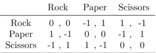
Normal-Form Games The real development of the field of game theory started with the work of Von Neumann and Morgenstern and their 1944 book [42]. In a game, players have to choose among a number of possible strategies, a combination of a strategy for each player gives an outcome, each player has her own preference concerning the possible outcomes. For Von Neumann and Morgenstern, the preferences are described in a matrix which for each combination of strategies, gives the integerpayoff of all players. This representation of the game is said to be innormal-form. Consider for example thepayoff matrix of the rock-paper-scissors game represented in Fig. 1.1. The actions of the first player are identified with the rows and the second player’s with the columns.

The first component in row r and column c corresponds to the payoff of the first player if she plays r and her opponent c, and the second component to the payoff of the second player. In rock-paper-scissors the payoffs of the players always sum up to 0, this is an instance of a two-playerzero-sum game, which was the object of the work of Von Neumann and Morgenstern. Such a game

(11)

is purely antagonistic, since players’preferences are opposed. A player tries to have the highest payoff, considering that the opponent is going to play the best counter-strategy. The strategy that ensures the best outcome in the worst case is called the optimal strategy. In zero-sum games, Von Neumann showed the existence of a pair of strategies, that is optimal, in the sense that each player minimizes her maximum loss [53]. In general, this requires mixed strategies, which allow randomization between several different actions. Therefore, the number of possible strategies is in fact infinite. For example in the rock-paper- scissors game, there are three pure strategies available, but the equilibrium is obtained by randomizing uniformly between these pure strategies.

Table 1.1: The game of rock-paper-scissors in normal-form.

Rock Paper Scissors Rock 0 , 0 -1 , 1 1 , -1 Paper 1 , -1 0 , 0 -1 , 1 Scissors -1 , 1 1 , -1 0 , 0

Nash equilibrium When games are not zero-sum, in particular when there are more than two players, winning strategies are no longer suitable to describe rational behaviors. In particular when the objectives of the players are not opposite, cooperation should be possible. Then, instead of considering that the opponent can play any strategy, we will assume that they are, also, rational. The notion of equilibria aims at describing rational behaviors. If we are expecting some strategy from the adversaries then it is rational to play the best response, that is the strategy that maximizes the payoﬀ if the strategies of the opponents are ﬁxed. The solution for non zero-sum games is a strategy for each player, such that knowing what the others are going to play, none of them is interested in changing her own. In other terms, each strategy is a best response to the other strategies.

For example consider the Hawk-Dove game, first presented by the biologists Smith and Price [48]. One such game is given in matrix form in Table 1.2. Two animals are fighting over some prey and can choose to either act as a hawk or as a dove. If a player chooses hawk then for the opponent the best payoff is obtained by playing dove. We say that dove is the best response to hawk.

Reciprocally the best response to dove is to play hawk. There are two “stable”

situations (Hawk,Dove) and (Dove,Hawk), in the sense that no player has an interest in changing her strategy.

Nash showed the existence of such equilibria in any normal-form game [44], which again requires mixed strategies. This result has revolutionized the field of economics, where it is used to analyze competitions between firms or gov- ernment economic policies for example. Game theory and the concept of Nash equilibrium are now applied to very diverse fields: in finance to analyze the evolution of market prices, in biology to understand the evolution of some species,

(12)

in political sciences to explain public choices made by parties.

Table 1.2: The Hawk-Dove game.

Hawk Dove Hawk 0 , 0 1 , 4 Dove 4 , 1 3 , 3

Games for Synthesis We aim at using the theory of non-zero-sum games for synthesizing complex systems in which several agents interact. Think for instance of several users behind their computers on a shared network. When designing a protocol, maximizing the overall performance of the system is de- sirable, but if adeviation can be proﬁtable to the users, it should be expected that one of them takes advantage of this weakness. This happened for example to the bit-torrent protocol where selﬁsh clients became more popular. Such de- viations can harm the global performance of the protocol. The concept of Nash equilibrium is particularly relevant, for one’s implementation to be used.

Unlike the ones we presented so far, in the context of controller synthesis, games are generally not presented in normal-form. Instead of being represented explicitly, it is more convenient to use games played on graphs. The graphs represent the possible conﬁgurations of the system. The controller can take actions to guide the system, and the system can also be inﬂuenced by the environment. Among games played on graph we can distinguish several classes.

The simplest one are turn-based games. For these games, in each state, one player decides alone on the next state. Inconcurrent games, in each state, the players choose their actions independently and the joint move formed by these choices determines the next state. Timed games are examples of concurrent games, which are played on timed automata. In a given state, several players can have actions to play, but only the player that moves ﬁrst has inﬂuence on the next state. Concurrent games and timed games are a valuable framework for the synthesis problem, we therefore chose to study the computation of Nash equilibria in this kind of games.

1.3 Examples

The examples we present now are going to be reused later, to illustrate the diﬀerent concepts that will be introduced. We describe the general ideas of the problems.

1.3.1 Peer to Peer Networks

In a peer-to-peer network clients share ﬁles that might interest other clients.

Clients want to download ﬁles from other clients but sending the ﬁles uses

(13)

bandwidth and prefer to limit this. The interaction in this situation could be modeled by a normal-form game, as is represented in Table 1.3 for two players.

To play this game, players have to choose independently if they are going to send or receive a file. An agent can only receive a file if another client is sending it. In this matrix game, the best response is never to send a file. However, this model is not accurate since in reality the situation is repeated. Considering that the game is repeated an infinite number of steps, players can take into account the previous actions of others to adapt their strategies. For instance, they can choose to cooperate and send the file in alternation. The tit-for-tat strategy, suggests that if one defects to send at his turn, the other stops as well. The best response is then to cooperate, since it gives a better accumulated payoff for both players.

Table 1.3: A game of sharing on a peer to peer network.

Receive Send Receive 0 , 0 2, -1

Send -1, 2 0, 0

1.3.2 Medium Access Control

This example was ﬁrst formalized from the point of view of game theory in [41]

Several users share access to a wireless channel. During each slot, they can choose to either transmit or wait for the next slot. The probability that a user is successful in its transmission decreases with the number of users emitting in the same slot. Furthermore each attempt at transmitting has its cost. The payoﬀ thus increases with the number of successful transmissions but decreases with the number of attempts. The expected reward for one slot and two players, is represented in Table 1.4, assuming a cost of 2 for each transmission, a reward of 4 for a successful transmission, a probability 1 to be successful if only one player emit, and of ¹₄ if they both transmit at the same time.

Table 1.4: A game of medium access.

Emit Wait Emit -1, -1 2, 0 Wait 0 , 2 0, 0

Once again, for a real situation, one step is not enough and there would be a succession of slots and the payoﬀ is then the accumulation of the payoﬀ for each slot. A better model will be presented in Section 2.1, Example 2.

(14)

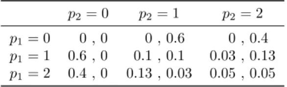
Table 1.5: Power control as a normal-form game p2= 0 p2= 1 p2= 2 p1= 0 0 , 0 0 , 0.6 0 , 0.4 p1= 1 0.6 , 0 0.1 , 0.1 0.03 , 0.13 p1= 2 0.4 , 0 0.13 , 0.03 0.05 , 0.05

1.3.3 Power Control in Cellular Networks

This game is inspired by the problem of power control in cellular networks.

Game theoretical concepts are relevant for this problem and Nash equilibria are actually used to describe rational behaviors of the agents [39, 40].

Consider the situation where a number of cellular telephones are emitting over a cellular network. Each agent Ai, can choose the emitting power pi of his phone. From the point of view of agentAi, using a stronger power results in a better transmission, but it is costly since it uses energy, and it lowers the quality of the transmission for the others, because of interferences. The payoﬀ for playerican be modeled by this expression from [47]:

R

pi 1−e^−0.5γⁱL

(1.1) whereγiis thesignal-to-interference-and-noise ratio for playerAi,Ris the rate at which the wireless system transmits the information in bits per seconds andL is the size of the packets in bits.

The interaction in this situation could be modeled by a normal-form game, as is represented in Table 1.5 for two players, three possible levels of emission and some arbitrary parameters. To play this game, players have to choose independently what power they will use, and the corresponding cell in the table gives the payoff for each of them. What would seem the best choice to maximize the total payoff of the player would be p1 = p2 = 1. However, knowing that playerA1 is going to choosep1, playerA2’s best response to maximize its own payoff is to choosep2 = 2. A better model for this problem, can be given as a repeated game, where at each step, each agentAican choose to increase or not its emitting powerpi. We will develop on this model in Section 2.1, Example 1.

1.3.4 Shared File System

We now take the example of a network file system. The problem occurs when several users have to share a resource. Several users on client computers can access the same files over a network, on a file server. The protocol for this file system can integrate file locking, like for instance NFS version 4. This prevents two clients accessing the same file at the same time. Such a protocol is said to be stateful, this is illustrated in Figure 1.1 for one lock and two clients. From

(15)

the initial configuration, one of the client can lock a file, and until it is not unlocked the file can not be accessed by others.

To perform some task, the clients access files on the system, and try to minimize the time until their task is completed. By maintaining a lock on a file they need later, they might lower the time necessary for their task, but this can have the opposite effect for other clients. We have to organize the accesses, so that clients are not tempted to act in an unpredicted way.

initial

locked by A1 locked by A2

A1 : lock A2 : lock

A1 : unlock A2 : unlock

Figure 1.1: A simple model of a shared ﬁle with one lock.

We will come back on this example in Section 2.1, Example 3.

1.4 Contribution

In this thesis we are interested in the existence and computation of Nash equilibria in games played on graphs. As several Nash equilibria may coexist, it is relevant to look for particular ones. It is interesting to look for Nash equilibria in pure strategies, since they can be implemented using deterministic programs.

It is also important to put constraints on the outcome of the equilibrium or on its payoff. We can for instance ask for an equilibrium where all players get their best payoff. Another constraint we allow, is on the actions used in the equilibria. We will see that the complexity of these different decision problems are closely related and lie most of the time in the same complexity classes.

Our approach consists in defining a transformation from multiplayer games to two-player zero-sum turn-based games. The search of Nash equilibria can now be seen as a antagonistic game in itself. Two-player zero-sum turn-based games have been much studied in computer science and efficient algorithms have been developed for synthesizing strategies, so that we can make use of them. With this transformation in mind, we study the complexity of finding Nash equilibria in finite concurrent games and treat classical objectives such as reachability, safety and other regular objectives. We describe the precise complexity class in which the problem lies for most of them. For instance, for Büchi objectives we show a polynomial algorithm to find equilibria, whereas for reachability objectives we show that the decision problems are^NP-hard.

These classical objectives are only qualitative, since players can either win or lose. To be more quantitative, we combine several objectives. We propose several ways to order the possible outcomes according to these multiple objectives. In general we use preorders, allowing to model some uncertainty about

(16)

the preferences of the players. To describe the preorders we use Boolean circuit.

We give an algorithm for the general case and analyze the complexity of some preorders of interest.

Finally, to allow for a more faithful representation of embedded systems we aim at analyzing timed games. We propose a transformation, based on regions, from timed to ﬁnite concurrent games, preserving Nash equilibria under some restriction on the allowed actions. We apply the techniques we developed so far to the obtained game. Our most general decision problem is EXPTIME- complete.

1.5 Related Works

Algorithmic game theory has dealt early with the problem of ﬁnding Nash equilibria in normal-form games. As they always exist if mixed strategies are allowed, this cannot be formulated as a decision problem, instead it is also possible to look at the problem as a search problem, Daskalakis, Goldberg and Papadimitriou showed that the total search problem of Nash equilibrium isPPAD-complete [19].

One interesting question is whether there exists an equilibrium with a particular payoﬀ, Gilboa and Zemel showed in 1989 that this question is NP-hard for normal-form games [25]. Another interesting problem is whether there exists a pure Nash equilibrium, Gottlob, Greco and Scarcello showed that this is NP-hard [27]. However these results consider a particular representation of the game in normal-form that is more succinct than the standard one. By contrast, in this work, we assume that the transition function of the game is given explicitly. For normal-form games, this means that the game is given as a matrix, in that case the existence of a pure Nash equilibrium is polynomial. Moreover, unlike normal-form games which are played in one shot, the games we consider are repeated, and are played on graphs.

A repeated game is basically a normal-form game, that is repeated for an inﬁnite number of steps, each player receiving an instant reward at each step.

An important result in the theory of repeated games, known as a folk theorem, is that any possible outcome can be an equilibrium given that all the players receive a payoﬀ above the minimal one they can ensure. This does not apply to the context we study since our games have internal states and players do not get instant reward. Instead their preferences depend on the sequence that is obtained in the underlying graph.

In games played on graphs, the number of pure strategies is inﬁnite, and Nash theorem no longer applies. The study of equilibria in graph games started by proving that in any turn-based game with Borel objectives, there exists a pure Nash equilibrium [14, 50]. In stochastic games, for some states, the successor is chosen randomly, according to a given probability distribution. In stochastic games where players take their actions simultaneously and independently at each step, Nash equilibria might not always exist. Instead, Chatterjee, Ma- jumdar and Jurdzi´nski showed that there areε-Nash equilibrium for reachability objectives [14] and any strictly positiveε. For quantitative objectives, in turn-

(17)

based games, Brihaye, Bruy`ere and De Pril showed the existence of equilibria, in games where players aim at minimizing the number of steps before reaching their objectives [10].

From the point of view of computer science, the existence of an equilibrium is not enough, we are interested in the complexity of ﬁnding a particular one.

Ummels studied the complexity of Nash equilibria for classical objectives in turn-based games. He showed that for Streett objectives the existence of Nash equilibria with constraints on the payoff isNP-complete while it is polynomial for Büchi objectives [49]. With Wojtczak, they showed that adding stochastic vertices makes the problem of finding a pure Nash equilibrium undecidable [51].

In a more quantitative setting, they also studied limit-average objectives in concurrent games. For these games, the existence of a mixed Nash equilibrium with a constraint on the payoﬀ is undecidable, while it isNP-complete when looking for pure Nash equilibria [52]. Klimos, Larsen, Stefanak and Thaarup, studied the complexity of Nash equilibria in concurrent games where the objective is to reach a state while minimizing some price. They show that the existence of a Nash equilibrium is^NP-complete [36]. It is to note that the model of concurrent games we study is slightly more general in that players do not observe actions.

This is sometimes called imperfect monitoring and has been discussed in other works [46, 18].

1.6 Outline

In Chapter 2, we deﬁne concurrent games which is the central model of games we are going to study. Together with this, we deﬁne the decision problems we are interested in: deciding if a player can ensure a given value, the existence of a Nash equilibrium, and the existence of a Nash equilibrium satisfying some constraints on its outcome and some constraints on the moves it uses. We also prove some basic properties, in particular undecidability in the general case, and possible translations from one decision problem to another.

In Chapter 3, we show how to transform a multiplayer concurrent game into a turn-based two-player game called the suspect game. This fundamental transformation relies on the central notion ofsuspect. We show that it is correct in the sense that ﬁnding a Nash equilibrium in the original game can be done by ﬁnding a winning strategy with some particular outcome in thesuspect game.

We also deﬁne a notion ofgame-simulation based on suspects, which preserves Nash equilibria.

In Chapter 4, we apply this transformation to ﬁnite games in order to describe the complexity of the diﬀerent decisions problem, for classical objectives.

In Chapter 5, we extend this result to a more quantitative setting, where each player has several objectives. We propose several ways to order the possible outcomes from these multiple objectives and analyze the complexity of the diﬀerent decision problems in each case.

In Chapter 6, we focus on timed games. We transform timed games into ﬁnite concurrent games, making use of a reﬁnement of the classical region abstraction.

(18)

We show a correspondence between Nash equilibria in the timed game and in the region game, and then analyze the complexity of our decision problems.

(19)

Chapter 2

Concurrent Games

In this chapter, we deﬁne the model of concurrent games formally, we present the concept of Nash equilibrium and the most relevant decision problems that arise from this notion. Finally, We give some generic properties of these diﬀerent problems in the context of concurrent games.

2.1 Definitions

A concurrent game corresponds to a transition system, over which the decision to go from one state to another is made jointly by players of the game. It is ﬁrst necessary to recall the essential vocabulary of transition systems and introduce the notations we will use.

Transition systems.Atransition system is a coupleS=hStates,Edgiwhere States is a set of states and Edg ⊆ States×States is the set of transitions.

Apath πinS is a sequence (si)0≤i<n (wheren∈N⁺∪ {∞}) of states such that (si, si+1)∈Edg for alli < n−1. Thelengthofπ, denoted by|π|, isn−1. The set of finite paths (also calledhistories) ofS is denoted by HistS, the set of infinite paths (also calledplays) ofSis denoted by Play_S, and PathS = HistS∪Play_S is the set of all paths ofS. Given a pathπ= (si)0≤i<n and an integerj < n: the j-th prefix ofπ, denoted byπ≤j, is the finite path (si)0≤i<j+1; thej-th suffix, denoted byπ≥j, is the path (sj+i)0≤i<n−j; thej-th state, denoted byπ=j, is the statesj. Ifπ= (si)0≤i<n is a history, we write last(π) =s_|π|for the last state ofπ. Ifπ^′ as a path such that (last(π), π^′₌₀)∈Edg, then theconcatenation π·π^′ is the pathρs.t. ρ=i=π=ifori≤ |π|andρ=i=π^′_{=(i−1−|π|)}fori >|π|. In the sequel, we write HistS(s), Play_S(s) and PathS(s) for the respective subsets of paths starting in state s, i.e. the paths π such that π=0 = s. If π is a play, Occ(π) = {s | ∃j. π=j = s} is the sets of states that appears at least once alongπand Inf(π) ={s| ∀i. ∃j≥i. π=j=s} is the set of states that appears infinitely often alongπ.

(20)

Players have preferences over the possible plays, and in a multiplayer games, this preferences are in general diﬀerent for each player. In order to be as general as possible, we describe these preferences as preorders over the possible plays.

We recall here, generic deﬁnitions concerning preorders.

Preorders.We fix a non-empty set P. A preorder over P is a binary relation.⊆P×P that is reflexive and transitive. With a preorder., we associate anequivalence relation ∼defined so thata∼bif, and only if, a.b andb.a.

Theequivalence class of a, written [a]_., is the set{b ∈ P | a ∼ b}. We also associate with. a strict partial order ≺deﬁned so that a≺b if, and only if, a.b and b6.a. A preorder.is said total if, for all elementsa, b∈P, either a.b, orb.a. An elementain a subsetP^′⊆P is saidmaximal inP^′ if there is no b ∈ P^′ such that a ≺ b; it is said minimal in P^′ if there is no b ∈ P^′ such thatb≺a. A preorder is saidNoetherian (orupwards well-founded) if any subsetP^′⊆P has at least one maximal element. It is saidalmost-well-founded if any lower-bounded subsetP^′ ⊆P has a minimal element.

We can deﬁne formally the games we are going to study.

Concurrent games [3].A concurrent game is a tuple G =hStates,Agt,Act, Mov,Tab,(-A)A∈Agti, where:

• States is a non-empty set ofstates;

• Agt is a ﬁnite non-empty set ofplayers;

• Act is a non-empty set ofactions, an element of Act^Agt is called amove;

• Mov : States×Agt → 2^Act\ {∅} is a mapping indicating the available actions to a given player in a given state, we say that a move mAgt = (mA)A∈Agt islegal atsifmA∈Mov(s, A) for allA∈Agt;

• Tab : States×Act^Agt→States is thetransition table, it associates, with a given state and a given move of the players, the state resulting from that move;

• for each A ∈ Agt, -A is a preorder over States^ω, called the preference relation of playerA, whenπ-Aπ^′, we say thatπ^′ isat least as good asπ forAand when it is not the case (i.e.,π6-Aπ^′), we say that Aprefers π overπ^′.

A finite concurrent game is a concurrent game whose set of state and actions are ﬁnite.

In a concurrent gameG, whenever we arrive at a states, the players simultaneously select an available action, which results in a legal movemAgt; the next state of the game is then Tab(s, mAgt). The same process repeatsad infinitum to form an inﬁnite sequence of states.

In the sequel, as no ambiguity will arise, we may abusively write G for its underlying transition system hStates,Edgi where Edg = {(s, s^′) ∈ States×

(21)

States | ∃mAgt ∈ Q

A∈AgtMov(A). Tab(s, mAgt) = s^′}. The notions of paths and related concepts in concurrent games follow from this identiﬁcation.

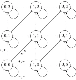
Example 1.As a ﬁrst example, we aim at modeling the power control problem described in Section 1.3.3. The arena on which the game is played is represented in Fig. 2.1 for a simple instance with two players: Agt ={A1, A2}, and three possible levels of emission. The set of states is States = [[0,2]]×[[0,2]], it corresponds to the current level of emission of the respective players: state (1,0) corresponds to player A1 using 1 unit of power and player A2 not emitting.

The two actions are to either increase one’s emitting power or to stick with the current one: Act = {+,=}. Transitions are labeled with the moves that trig- ger them, for instance there is a transition from (0,0) to (1,0) labeled byh+,=i, meaning that if playerA1choose action+and playerA2action=, the game goes from (0,0) to (1,0): formally Tab((0,0),(+,=)) = (1,0). Allowed actions from a state are deduced from the label on outgoing edges, for instance in (2,2) the only outgoing edge is labeled byh=,=i, so Mov((2,2), A1) = Mov((2,2), A2) ={=}.

We do not deﬁne a preference relation yet, but in the following we will see many practical ways to deﬁne these.

0,0 0,1

1,0 0,2

1,1

2,0 1,2

2,1 2,2

=,+

+,= +,+

=,=

Figure 2.1: A simple game-model for the power control in a cellular network

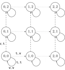
Example 2.As a second example, we model the problem of medium access control described in Section 1.3.2. The arena on which the game is played is represented in Fig. 2.2 for a simpliﬁed instance with two players: Agt = {A1, A2}. The set of states States = [[0,2]]×[[0,2]] corresponds to the number of successful frames that players have transmitted so far, and assuming they have a total of 2 frames to transmit. The two actions are to either transmit or wait:

(22)

0,0 0,1

1,0 0,2

1,1

2,0 1,2

2,1 2,2

w,t

t,w t,t w,w

Figure 2.2: A simple game-model for the medium access control

Act ={t,w}. If the two players attempt to transmit at the same time then no frame is received.

Example 3.As a third example, we model the problem of shared ﬁle system described in Section 1.3.4. The arena on which the game is played is represented in Fig. 2.3 for an instance with two players: Agt ={A1, A2} and two ﬁles F1

andF2 that are shared.

Strategies.Let G be a concurrent game, and A ∈ Agt. A strategy for A maps histories to available actions, formally it is a function σA: HistG → Act such that σA(π) ∈ Mov(last(π), A) for all π ∈ HistG. A strategy σP for a coalitionP ⊆Agt is a tuple of strategies, one for each player inP. We write σP = (σA)A∈P for such a strategy. A strategy profile is a strategy for Agt.

We write Strat^P_G for the set of strategies of coalitionP, and ProfG = Strat^Agt_G . Outcomes.LetGbe a game,P a coalition, andσP a strategy forP. A pathπ iscompatible with the strategy σP if, for all k <|π|, there exists a movemAgt

such that

1. mAgt is legal atπ=k,

2. mA=σA(π≤k) for all A∈P, and 3. Tab(π=k, mAgt) =π=k+1.

We write OutG(σP) for the set of paths in G that are compatible with strat- egyσP ofP, these paths are calledoutcomesofσP. We write Out^f_G(σP) (resp.

(23)

F1 locked byA1

F2 locked byA1

F1 locked byA1

F2 locked byA1

F1 locked byA1

F2 locked byA2

initial

F1 locked by A2

F2 locked by A1

F2 locked byA2

F1 locked by A2

F2 locked by A2

lockF2,w

unlockF1,w w, lockF1

w,w

Figure 2.3: A game-model for a network ﬁle system.

Out^∞_G (σP)) for the ﬁnite (resp. inﬁnite) outcomes, and OutG(s, σP), Out^f_G(s, σP) and Out^∞_G(s, σP) for the respective sets of outcomes of σP with initial state s.

Notice that any strategy profile has a single infinite outcome from a given state, thus when given a strategy profile σAgt, we identify OutG(s, σAgt) with the unique play it contains. When G is clear from the context we simply write Out(s, σAgt) for OutG(s, σAgt).

Note that, unless explicitly mentioned, we only consider pure (i.e., non- randomized) strategies. Notice also that strategies are based on the sequences of visited states, and not on the sequences of actions played by the players.

This is realistic when considering multi-agent systems, where only the global eﬀect of the actions of the agents is assumed to be observable. Being able to see (or deduce) the actions of the players, would make the various computations easier. When we can infer from the transition that was taken, the actions of all players, we call the gameaction-visible, formally this is when Tab(s, mAgt) = Tab(s, m^′_Agt) if, and only if,mAgt=m^′_Agt. A particular case of an action-visible game is the classical notion ofturn-based game, a game is said to beturn-based if for each statesthe set of allowed moves is a singleton for all but at most one

(24)

playerA, this playerA is said tocontrol that state, and she chooses a possible successor for the current state, i.e. Act = States and Tab(s, mAgt) =s^′ if, and only if,mA=s^′.

Example 4.For example, the game we used in Example 2 to model medium access control, represented in Fig. 2.2, is not action-visible: if the game stays in the same state, it is not possible to know if it is because both players have waited or if it is because there was a collision when they tried to transmit. On the other hand, the game of Example 2.1 modeling power control, is action- visible since two diﬀerent legal moves will always lead to two diﬀerent states.

We give an example of a turn-based game in Fig. 2.4.

s0

s1

s2

s3

s4

s5

A1

A2

A3

Figure 2.4: A simple turn-based game. It is convenient to use a diﬀerent representation for this class of game: instead of labeling the edges with actions, we denote below each state, which player is controlling that state, so in that case player A1 controls state s0, player A2 controls state s1 and player A3 controls states2.

2.2 Value and Nash Equilibria

A concurrent game involving only two players (AandB, say) iszero-sumif, for any two playsπandπ^′, it holdsπ-_Aπ^′if, and only if,π^′-_Bπ. Such a setting is purely antagonistic, as both players have opposite preference relations. The most relevant concept in such a setting is that ofoptimal strategies where one player has to consider the strategy of the opponent that is the worst for her, while trying to ensure the maximum possible with respect to her preference.

The minimum outcome she can get if she plays optimally is called her value.

This is a central notion in two-player games since the minimax theorem of Von Neumann [53], but it is also applicable in the context of multi-player games.

(25)

Value.Give a gameG, we say that a strategyσAforAensuresπfromsif every outcome ofσAfromsis at least as good asπforA, i.e.∀π^′ ∈Out^∞_G(s, σA). π-A

π^′. We also say that A can ensure π when such a strategy σA exists. A value of game G for playerA from a state s is a maximal element of the set of paths that player A can ensure, i.e. it is a path π such that there is σA,

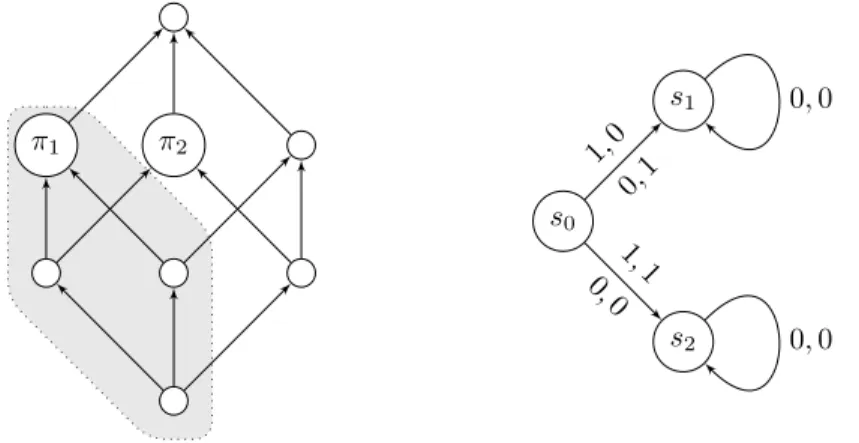
∀π^′∈Out(s, σA). π-Aπ^′.

Remark. When preference relations are described by preorders, their might be incomparable values. Consider for example the turn-based game whose arena is represented in Fig. 2.4, and with a preference relation for playerA1given by the preorder represented in Fig. 2.5. By choosings1,A1 can ensures0·s1·s4, and by choosings2she can ensures0·s2·s4, but she cannot ensure a path that is at least as good as both: these are two incomparable values, which ares0·s1·s4

ands0·s2·s4.

s0·s1·s4 s0·s2·s4

s0·s1·s3

s0·s2·s5

Figure 2.5: An example of a preference relation for the arena of Fig. 2.4. There is an edgeπ1→π2 whenπ1≺π2. With this preference relation, playerA1 has two incomparable values.

The decision problem associated to the notion of value is called the value problem and is deﬁned as follow:

Value problem:Given a gameG, a statesofG, a playerAand a playπ, can A ensure π from s (i.e. is there a strategy σA for player A such that for any outcomeρ∈Out^∞_G (s, σA), it holdsπ-Aρ)?

In non-zero-sum games, optimal strategies are usually too restricted since they consider that one player always plays against all the others. More relevant concepts areequilibria, which correspond to strategies on which the players can agree. One of the most studied notion of equilibria isNash equilibria, in which the strategy of any player is optimal assuming the strategy of the others are ﬁxed. We now introduce this concept formally.

Nash equilibria.LetGbe a concurrent game and let sbe a state ofG. Given a movemAgt and an actionm^′ for some playerA, we writemAgt[A7→m^′] for the move nAgt with nB =mB when B 6=A and nA = m^′. This is extended to strategies in the natural way. A Nash equilibrium [44] of G from s is a

(26)

strategy proﬁleσAgt ∈ProfG such that for all playersA∈Agt and all strategies σ^′∈Strat^A:

Out(s, σAgt[A7→σ^′])-AOut(s, σAgt)

In that contextσ_A^′ is called adeviation due toA, andAis called adeviator.

π1 π2

Figure 2.6: The notion ofimprovement for a non-total order.

s0

s1

s2

1,0 0,1

0,0 1,1

0,0 0,0

Figure 2.7: Example of a concurrent game with no pure Nash equilibrium Hence, Nash equilibria are strategy proﬁles where no single player has an incentive to unilaterally deviate from her strategy.

Remark. The definition of Nash equilibria we have chosen, allows to model uncertainty about the preferences of players, by giving a partial order for the preferences. For instance for the preorder of Fig. 2.6, the fact that it is not known whether the player prefersπ1orπ2, is modeled by these two paths being incomparable. We have to consider that π2 is a possible improvement of π1, and also that π1 possibly improve π2. If we want this player to play a Nash equilibrium whose outcome is π1 we have to ensure that if she changes her strategy, the outcome will still be in the gray area. We can in fact notice that a Nash equilibrium for a preference relations-_Agt, is also a Nash equilibrium for all preference relations which refine-_Agt: formally-^′ refines-if for all paths πandπ^′,π-π^′ impliesπ-^′π^′; then ifσAgtis a Nash equilibrium, then for all player A and strategy σ_A^′ : Out(s, σAgt[A7→ σ^′]) -_A Out(s, σAgt), therefore if -^′_A refines-_A, Out(s, σAgt[A7→σ^′])-^′_AOut(s, σAgt), and σAgt is also a Nash equilibrium if we replace the preference relation-Agt by-^′_Agt.

Remark. Although we restrict our strategy to pure strategies, a pure Nash equilibrium is resistant to mixed strategies.

Remark. In concurrent games, when we restrict strategies to pure one there might not always be a Nash equilibrium. For example, in the game represented in Fig. 2.7 and called the matching pennies, we consider that playerA1prefers

(27)

to reach states1 while playerA2 prefers to reach states2. If the strategies are ﬁxed, then one of the two players can change her strategy in order to reach the state she prefers. Hence, starting from states0, there is no Nash equilibrium with pure strategies in that game.

Since they do not always exist, the basic question about Nash equilibria, is whether there exist one in from given game. We will formulate this question as a decision problem.

Existence problem:Given a game G and a state s in G, does there exist a Nash equilibrium inG froms?

Deciding if there exists a Nash equilibrium, is often not enough, as several can coexist and there might exist one that is better for everyone than some other.

Thus we reﬁne the existence problem by adding constraints on the outcome.

For instance we can ask if there is a Nash equilibrium whose outcome is the best for every player. The constraint on outcomes will be given by two plays π_A⁻ and π_A⁺ for each player A∈Agt, giving respectively a lower and an upper bound for the desired outcome. When the outcomeπof a strategy proﬁleσAgt

satisﬁesπ⁻_A-Aπ-Aπ_A⁺for allA∈Agt, we say thatσAgt satisfies the outcome constraint(π⁻_A, π_A⁺)A∈Agt.

Existence with constrained outcomes:Given a game G, a state s in G, and two playsπ⁻_A and π⁺_A for each player A, does there exist a Nash equilibrium σAgt in G from s satisfying the outcome constraint (π_A⁻, π⁺_A)A∈Agt (i.e.

π_A⁻-AOut(s, σAgt)-Aπ_A⁺ for allA∈Agt)?

In some situations, we also want to restrict the moves that are used by the strategies of the equilibria. For design reason, we might want to restrict the number of actions we are going to use, in order for the strategy to be simpler to implement. But we still want to be resistant to actions outside of the one we chose. The constraint on the move will be formally given by a function Allow : (States×Act^Agt) → {true,false}. When Allow(s, mAgt) = truewe say that the movemAgt isallowedins. When a strategy proﬁleσAgtis such that for any historyh, Allow(last(h), σAgt(h)) =true, we say thatσAgt satisfy the move constraintAllow. This leads to the decision problem with constrained moves:

Existence with constrained moves:Given a game G = hStates,Agt,Act, Mov,Tab,(-A)A∈Agti, a states∈States, two playsπ_A⁻andπ_A⁺for each playerA, a function Allow : (States×Act^Agt)→ {true,false}, does there exist a Nash equi- libriumσAgt in G froms satisfying the outcome constraint (π_A⁻, π_A⁺)A∈Agt and the move constraint Allow (i.e. for any historyhfroms, Allow(last(h), σAgt(h)) = true) ?

In the following when talking about the constrained existence problem, we will refer to the existence with constrained moves which is the most general problem. It is clear that if we can solve the existence with constrained move we

(28)

can also solve the existence with constrained outcome, and if we can solve the existence with existence with constrained outcome we can solve the existence problem.

When studying the complexity of this problem, we will restrict the func- tions Allow given as input to the ones that are computable in polynomial time.

To ensure this we could for example ask for a function given by a Boolean circuit. We now see an example of such a constraint Allow, we will also see in Chapter 6, that this constraint is useful when interpreting timed games as concurrent games, to decide the existence problem.

Example 5.In a real situation, involving several similar devices, it would be more practical if all devices run the same program. When the situation is modeled as a game, this means that the strategy should to be the same for all players. Assuming they are synchronous, we can make use of the constraint on moves. We enforce the restriction with the function deﬁned by Allow(s, mAgt) if and only ifmA=mB for any players A, B∈Agt.

The complexity of all these decision problems heavily depends on what preorders we allow for the preference relation and how they are represented. Even for ﬁnite games, in their most general form, all these problems are undecidable, as we prove in the next section.

2.3 Undecidability in Weighted Games

A weighted game is a standard concurrent game where preference for each playerAis given by aweight functioncostA: States7→Z. Theaccumulated cost of playρis given by the sum of the weights: costA(ρ) =P

i≥0costA(ρi). The goal of the player is then to minimize the accumulated cost. Formally, forρand ρ^′two plays,ρ-Aρ^′if, and only if,costA(ρ) is ﬁnite andcostA(ρ)≤costA(ρ^′) orcostA(ρ^′) is inﬁnite.

Theorem 2.1. The existence and constrained-existence problems are undecidable for weighted games.

Proof. We ﬁrst prove the result for the constrained existence problem. We encode the halting problem for two-counter machines into a turn-based weighted game with 5 players. This problem is known to be undecidable. Without loss of generality, we will assume that the two counters are reset to zero before the machine halts. The value of counterc1 is encoded in the following way: if its value isc1for a given history of the two-counter machine, then the accumulated cost for playerA1 of the corresponding history is c1−1 and the accumulated cost forB1 is−c1. Having two players for one counter will make it easy to test whether it equals 0. Similarly to code the value of c2, we have one playerA2

whose accumulated cost is equal toc2−1 andB2whose accumulated cost is equal to−c2. To initialize the value of the counter, we visit a state whose weight is−1 forA1 andA2 before going to the initial state. And we do the opposite in the

(29)

q C

u1 q^′ A1

u0 q^′′

B1

. . .

Figure 2.8: Testing whether c1= 0.

halting state so that in a normal execution the accumulated weight for allAiand Biis 0. Incrementing counterci, consists in visiting a state whose weight is 1 for Aiand−1 forBi, and vice versa for decrementing this counter. More precisely, if instruction qk of the two-counter machine consists in incrementing ci and jumping toqk^′, then the game will have a transition from stateqk to a statepk

whose weight is given bycostAi(pk) = 1,costBi(pk) =−1, andcostA(pk) = 0 for a playerA∈Agt\ {Ai, Bi}, and another transition from there toqk^′.

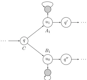
It remains to encode the zero-test, for this the game will involve an additional playerC, the aim of this player will be to reach the state corresponding to the ﬁnal state of the two-counter machine, this is encoded by giving a negative cost forCto the state of the game corresponding to the ﬁnal state of the two-counter machine. The equilibrium we will ask for, is one whereCreaches her goal, and A1,A2,B1 and B2 gets an accumulated cost of 0. Now, a zero-test is encoded by a module shown in Fig. 2.8. In this module, playerC will try to avoid the two sink states (marked in grey), since this would prevent her from reaching her goal.

When entering the module, player C has to choose one of the available branches: if she decides to go tou1, thenA1 could take the play into the self- loop, which is an improvement for her if her accumulated cost in the history is below 0, which corresponds to havingci= 0; hence playerC should play tou1

only ifc16= 0, so that A1will have no interest in going to this self-loop.

Similarly, if playerC decides to go tou0, playerB1 has the opportunity to

“leave” the main stream of the game, and go to the sink state. If the accumulated cost for B1 is below 0 up to that point, corresponding to a value of c1

strictly positive, then B1 has the opportunity to play in the self-loop, and to win. Conversely, whenc1= 0,B1has no interest in playing in the self-loop since her accumulated cost would be 0. Hence, ifci = 0 when entering the module,

(30)

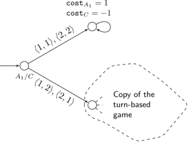
A1/C

Copy of the turn-based game h1,1i,h2,2i

h1,2i,h2,1i cost_A

1 = 1 cost_C=−1

Figure 2.9: Extending the game with an initial concurrent module

then playerC should go tou0.

One can then easily show that the 2-counter machine stops if, and only if, there is a Nash equilibrium in the resulting game, in which playerC reach her goal and players A1, B1, A2 and B2 have an accumulated cost of 0. Indeed, assume that the machine stops, and consider the strategies where playerCplays (in the first state of the test modules) according to the value of the corresponding counter, and where players A1, B1, A2 and B2 always keep the play in the main stream of the game. Since the machine stops, player C wins, while players A1, B1, A2 and B2 get an accumulated cost of 0. Moreover, none of them has a way to improve their payoff: since playerC plays according to the values of the counters, playersA1andA2would not benefit from deviating from their above strategies. Conversely, if there is such a Nash equilibrium, then in any visited test module, playerC always plays according to the values of the counterci: otherwise, playerAi (orBi) would have the opportunity to win the game. By construction, this means that the outcome of the Nash equilibrium corresponds to the execution of the two-counter machine. As player C wins, this execution reaches the final state.

We can prove hardness for the existence problem as well, by adding a module as represented in Fig. 2.9. There exists a Nash equilibrium in this game if and only if there is one whereC reaches her goal in the turn-based game. We will use the idea of this module several time in the following. In the next section, we will provide a generic lemma that generalizes this idea.

2.4 General Properties

This section contains generic lemmas that we reuse several times later.

(31)

2.4.1 Nash Equilibria as Lasso Runs

We ﬁrst characterize outcomes of Nash equilibria as ultimately periodic runs in ﬁnite games.

Lemma 2.2. Letsbe a state of a finite game G. Assume that every player has a preference relation which only depends on the set of states that are visited and on the set of states that are visited infinitely often (in other terms, ifInf(ρ) = Inf(ρ^′)andOcc(ρ) = Occ(ρ^′), thenρ∼Aρ^′ for every player A∈Agt).

If there is a Nash equilibrium with outcomeρ, then there is a Nash equilibrium with outcomeρ^′ of the formπ·τ^ω such thatρ∼Aρ^′, and where|π|and|τ|

are bounded by|States|².

Proof.LetσAgt be a Nash equilibrium, andρbe its outcome froms. We deﬁne a new strategy proﬁle σ_Agt^′ , whose outcome from s is ultimately periodic, and then show thatσ^′_Agt is a Nash equilibrium froms.

To begin with, we inductively construct a historyπ=π0π1. . . πn that is not too long and visits precisely those states that are visited byρ.

The initial state is π0 = ρ0 = s. Then we assume we have constructed π≤k =π0. . . πk which visits exactly the same states as ρ≤k^′ for somek^′. If all the states ofρhave been visited inπ≤kthen the construction is over. Otherwise there is an indexisuch thatρidoes not appear inπ≤k. We therefore deﬁne our next target as the smallest suchi: we let t(π≤k) = min{i | ∀j ≤k. πj 6=ρi}.

We then look at the occurrence of the current stateπk that is the closest to the target inρ: we letc(π≤k) = max{i < t(π≤k)|πk=ρi}. Then we emulate what happens at that position by choosingπi+1=ρc(π≤i)+1. Thenπi+1 is either the target, or a state that has already been seen before inπ≤k, in which case the resultingπ≤k+1 visits exactly the same states asρ≤c(π_≤i)+1.

At each step, either the number of remaining targets strictly decreases, or the number of remaining targets is constant but the distance to the next target strictly decreases. Therefore the construction terminates. Moreover, notice that between two targets we do not visit the same state twice, and we visit only states that have already been visited, plus the target. As the number of targets is bounded by |States|, we get that the length of the pathπ constructed thus far is bounded by 1 +|States| ·(|States| −1)/2.

Using similar ideas, we now inductively construct τ = τ0τ1. . . τm, which visits precisely those states which are seen infinitely often along ρ, and which is not too long. Letl be the least index after which the states visited byρare visited infinitely often: l = min{i | ∀j ≥i. ρj ∈Inf(ρ)}. The runρ≥l is such that its set of visited states and its set of states visited infinitely often coincide.

We therefore deﬁneτin the same way we have deﬁnedπabove, but for playρ≥l. As a by-product, we also getc(τ≤k), fork < m.

We now need to glueπandτ together, and to ensure thatτ can be glued to itself, so thatπ·τ^ω is a real run. We therefore need to link the last state ofπ with the first state ofτ(and similarly the last state ofτwith its first state). This possibly requires appending some more states toπandτ: we fix the target ofπ andτ to beτ0, and apply the same construction as previously. The total length

(32)

We let ρ^′ = π·τ^ω, and abusively write c(ρ^′_≤k) for c(π≤k) if k ≤ |π| and c(τ≤k^′) with k^′ = (k−1− |π|) mod|τ| otherwise. We now deﬁne our new strategy proﬁle, havingρ^′ as outcome from s. Given a historyh:

• if hfollowed the expected path, i.e., h=ρ^′_≤k for some k, we mimic the strategy at c(h): σ_Agt^′ (h) = σAgt(ρc(h)). This way, ρ