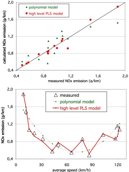
A set of 3 real driving cycles, the so-called Artemis cycles, were designed to be representative of European driving behaviour. 3 emission models have been designed, at best accurate for any driving behavior: one based on the instantaneous speed (after an emission signal inverse modelling), one according to the distribution of the instantaneous speed and acceleration, and a third according to seven dynamic related parameters.
INTRODUCTION
Many of the parameters that affect emission measurements are well known, but their actual impact on results has not been well quantified. It should also try to improve the understanding of the effects that these parameters can have on the measured emissions.
METHODOLOGY
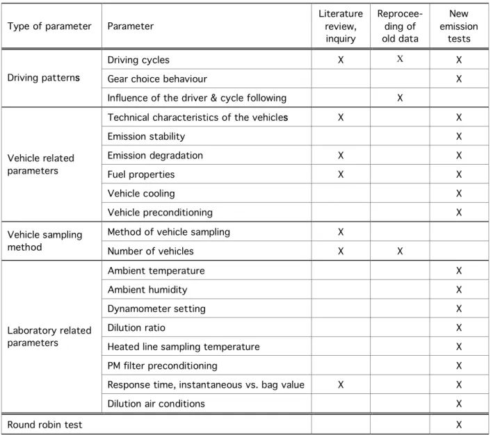
P ARAMETERS STUDIED
- Pollutants considered
- Parameters of the measurement accuracy
The effect of sample size on average emissions for different types of vehicles is studied by a statistical investigation of existing databases. The impact on ambient air emissions used to dilute the raw gas in the CVS can be non-negligible.
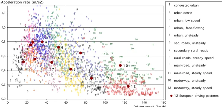
B UILDING OF THE A RTEMIS DRIVING CYCLES
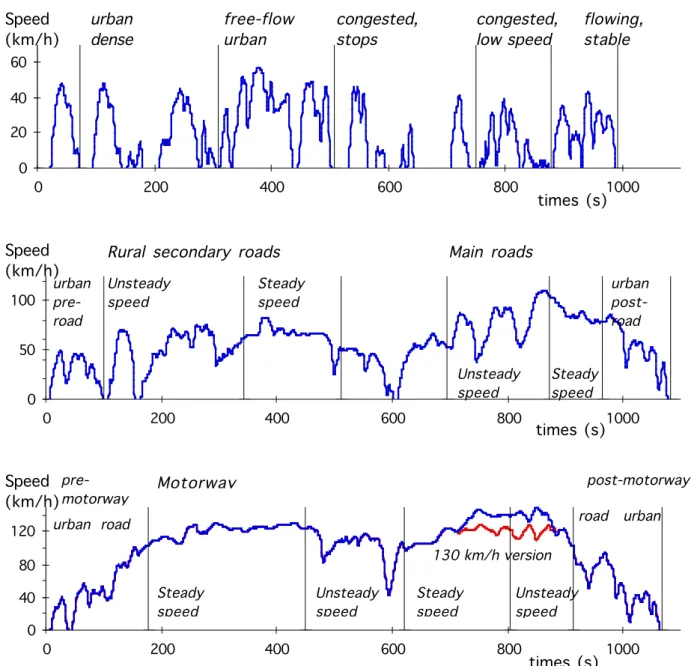
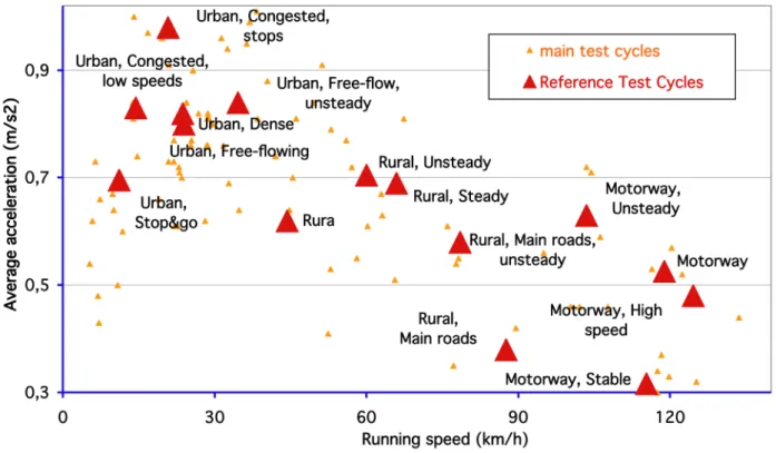
The cycle structure was determined according to the composition of the actual trips taking into account the 12 typical driving conditions. This weighting, given in (André, 2004a, b), is based on the observed statistics and share of the different driving patterns and trip categories.
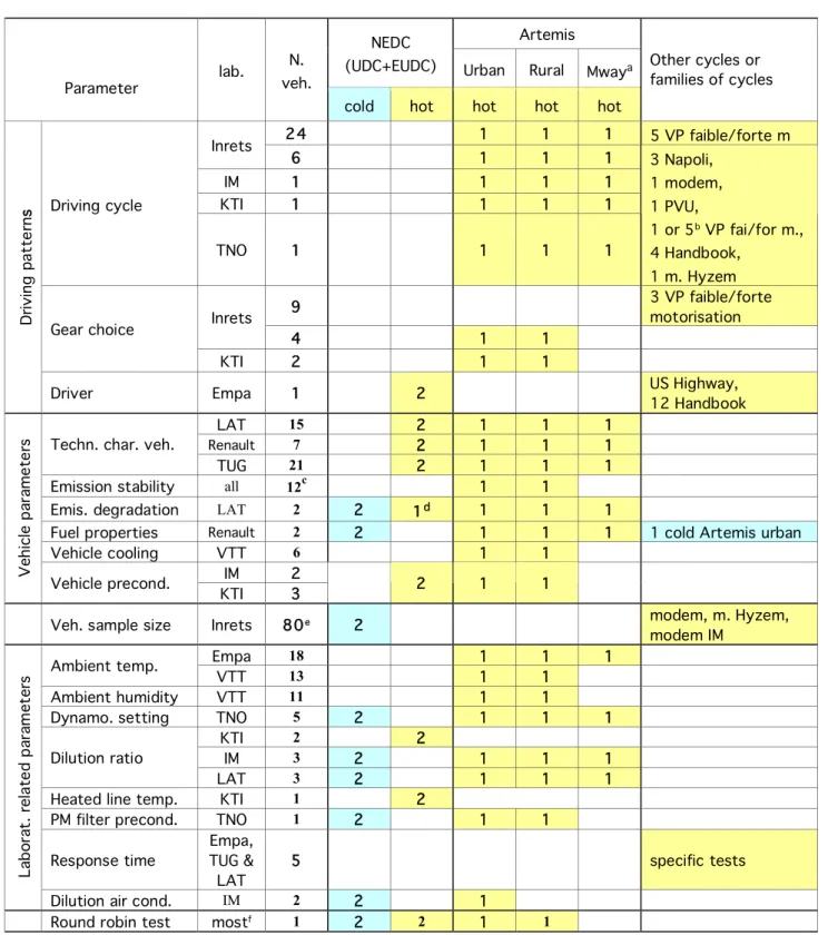
D ESCRIPTION OF THE EMISSION TESTS
- List of driving cycles used
- Test sequences
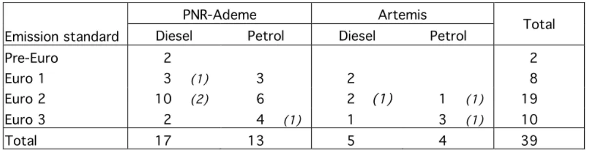
- Vehicle sample
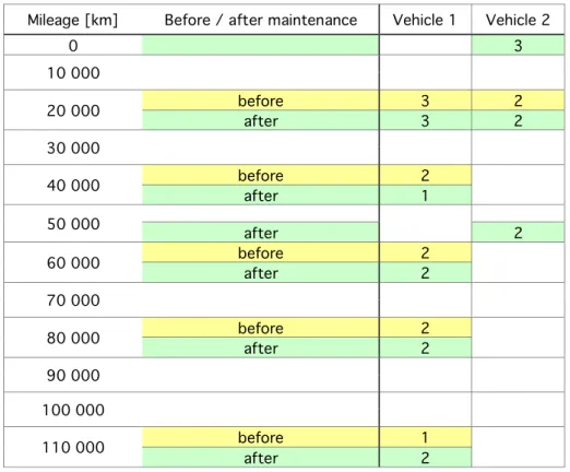
The second part of the test sequence is similar to the sequence but performed with the Artemis rural driving cycle (Cornelis et al., 2005). In another vehicle, it was possible to obtain a reference measurement at 0 km.
S PECIFIC METHODS AND METHODS OF DATA PROCESSING
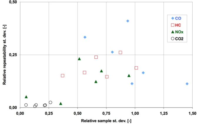
- Short term emission stability
- Selection of the fuels tested
- Methods of vehicle sampling
- Minimum vehicle sample size
- Response time, including instantaneous vs. bag value
- Round robin test
We then considered all intermediate vehicle sample sizes between one and the full sample size. Explanation of the change of the emission value from their place of formation to the analyzer signal using formulas.

DETAILED RESULTS
D RIVING PATTERNS
- Driving cycles
- Gear choice behaviour
- Influence of the driver and of the cycle following
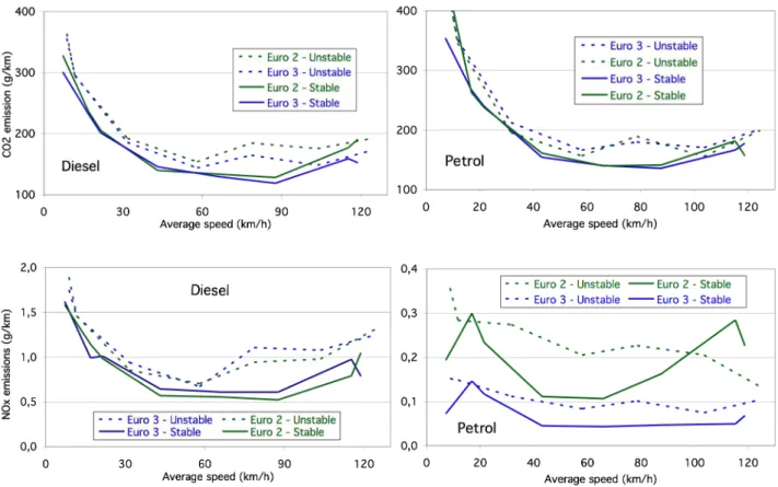
A specific analysis was performed to instead highlight the sensitivity of the emission to the test protocol: i.e. Relative variation ranges are provided according to the standard deviation of the relative emissions (Table 12). We conclude that, for the recent vehicles (Euro 2 and 3), the use of one unique set of driving cycles (such as the Artemis cycles) leads to a significant underestimation (by 15 to 20 %) of the CO (petrol ) and of the HC and particles (diesel), and to an overestimation of the diesel CO (at 20.
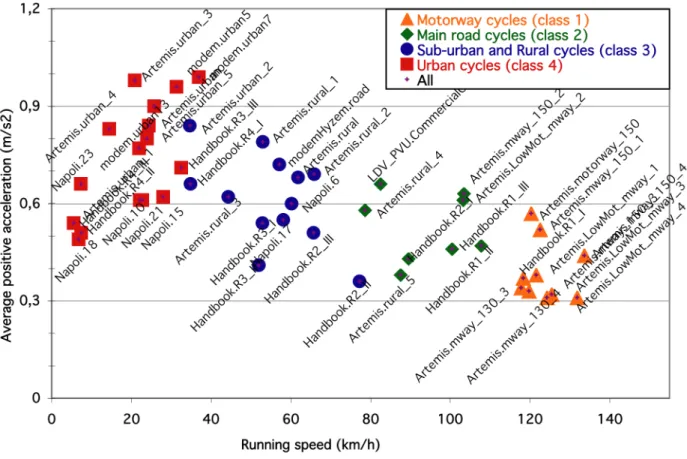
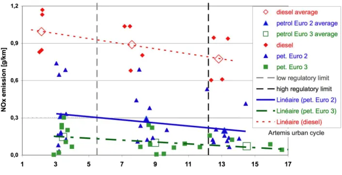
The significant impact of driving conditions on emissions means a necessary correction of this heterogeneous data set in terms of the driving cycle. These reference emissions should then be used to calculate emission factors and develop modeling approaches. For cars, the 2-dimensional distribution of velocity and acceleration is calculated for these velocity curves.
The tests used for the analysis of the robot and human drivers were performed with a tolerance band of ± 2 km/h and ± 1 s.

V EHICLE RELATED PARAMETERS
- Technical characteristics of the vehicles
- Short term emission stability
- Long term emission degradation
- Fuel properties
- Vehicle cooling
- Vehicle preconditioning
Similarly for HC and CO, also no impact of emission control technology is evident for the cars tested here. This impact of aromatic content is offset by other Artemis cycles run under hot start conditions. However, and regardless of what was predicted by the EPEFE formulas, it is clear that fuel composition has an impact on HC emissions.
For NOx, the influence of the aromatic content is similar to that for CO and HC. The emission test results of diesel cars are affected by preconditioning to a lesser extent than those of the petrol vehicles. This is partly due to the fact that the first part of the NEDC cycle can be considered a kind of preconditioning.
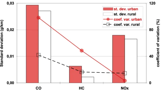
It resulted in the lowest emission levels and the lowest standard deviation for the majority of measurements.
V EHICLE SAMPLING METHOD
- Method of vehicle sampling
- Minimum vehicle sample size
This list contains all the characteristics of the vehicles sold and the coordinates of the owner. The laboratory sends a letter to all owners of the desired vehicle (at least 100 letters to ensure sufficient positive responses). The coordinates of the owners and the technical characteristics of the vehicle are obtained by advertising to the staff of the laboratory company and of surrounding companies.
When selecting the vehicle category, it is often possible to choose between several vehicles. All labs reject vehicles with serious defects such as a broken exhaust pipe, lack of basic equipment. The methodology followed allows the determination of the minimum number of vehicles, or the minimum sample size, necessary to obtain the same quality of an emission model according to the average cycle speed than with the maximum size of the studied sample (Lacour & Joumard, 2001).
In this case, the entire sample converges, but it is not necessary that the average of the entire sample converges to a constant value.

L ABORATORY RELATED PARAMETERS
- Ambient air temperature
- Ambient air humidity
- Dynamometer setting
- Exhaust gas dilution ratio
- Heated line sampling temperature
- PM filter preconditioning
- Response time, including instantaneous vs. bag value
- Dilution air conditions
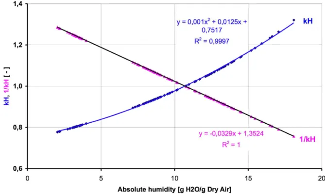
The influence of ambient temperature on emissions was in most cases linear (see an example Figure 17), but in some cases (urban HC for Euro 4 petrol and highway HC for Euro 2 diesel), the exponential type of function provided a better fit. The humidity effect can be normalized according to a reference point, chosen as for the existing correction factor (see an example in figure 19): It corresponds to an actual correction factor kH equal to 1, i.e. deviations from -12 to -4 % were observed for the results of the minimum settings compared to the average settings.
Deviations of +2 to +25% have been observed for the results of the maximum settings compared to the average settings. However, a clear trend was observed for the NOX emissions from diesel-powered passenger cars. The very small size of the vehicle samples (3 petrol, 2 diesel cars) does not allow a clearer conclusion.
The results show that no effect of PM filter conditioning temperature and relative humidity was observed during the tests (Geivanidis et al., 2004): See Figure 24.
R OUND ROBIN TEST
Two sets of repetitions took place at the beginning, and the third set at the end of the round robin test. Furthermore, closer assessment of the data shows that it was not possible to develop any. Therefore, it was likely that the results measured in this round-robin exercise were different from those that would have been obtained if the round-robin test had been carried out in parallel with the actual test itself.
However, the consortium had no provisions to perform that task, as the round was part of the extension, not part of the original agreement, and the extension was long delayed by the contractual dispute. Only if each of the pollutants were considered separately could one find some cases where a laboratory's results for that particular pollutant over all the cycles tested could be consistently higher or lower than the average. This can be seen in Figure 27 which shows the average variation (all cycles and all components) for each laboratory, with the high-low bars marking the largest deviations.
Even in those labs that appear to average above or below the group mean, the high or low ends of the columns extend to the other side of the 0-axis, indicating that overestimation (or underestimation) was not consistent.
SYNTHESIS AND CORRECTION FACTORS
- N OT INFLUENCING PARAMETERS
- P ARAMETERS WITH QUALITATIVE INFLUENCE
- I NFLUENCING PARAMETERS
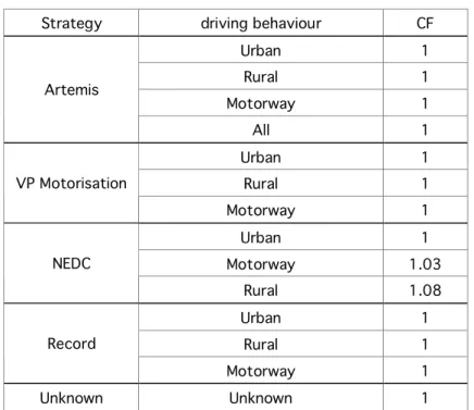
- C ORRECTION FACTORS
Under these described figures, the weighting of the individual behavior of several vehicles is very important to obtain an average, which is representative of an average behavior. Analyzes of emissions related to driving cycles have shown their significant impact (and often overriding other factors such as vehicle category or fuel). Given the very high diversity of emissions data collected in the Artemis database - and the large range of relevant driving cycles - it was however not possible to elaborate on the emission factors without managing the impact of this cycle.
This "test cycle mapping" then enabled the hot emission data to be aggregated into coherent clusters. The impact of mileage on fuel vehicle emissions depends on the pollutant, type approval category (or emission standard) and average speed. The effect of ambient temperature is available for all pollutants and most vehicle classes.
The influence of ambient humidity only exists for NOx and for some vehicle classes.
GUIDELINES
- V EHICLE SAMPLING
- U SAGE CONDITIONS OF THE VEHICLES
- Driving cycle
- Gearshift strategy
- Vehicle preconditioning
- Driver
- Fuel characteristics
- Ambient air temperature and humidity
- Vehicle cooling
- Dynamometer setting
- S AMPLING AND ANALYSING THE POLLUTANTS
- D ATA MANAGEMENT
The Artemis cycles do not depend on the performance of the vehicle, but similar cycles are adapted to the performance of the vehicle. It is therefore recommended to measure the emissions close to the average ambient temperature rather than at the "standard", when this is far from reality. Again, therefore, whenever possible, it is recommended to perform the tests with an ambient humidity close to the real-world average.
This may be due to the small sample size and the widely standardized sampling and analysis conditions respected by the participating laboratories. Nevertheless, the contaminant analysis and sampling conditions appear to be by far an important source of error compared to the other parameters examined above. Accurately record the characteristics of the vehicle, the conditions of use of the vehicle as mentioned above (driving cycle characteristics, ambient air, cooling..), especially when these conditions are stable in the laboratory, but also specific to the laboratory.
Do not apply any correction factor to the measured parameters, especially regarding the air humidity.
CONCLUSION
The status of the tested vehicles according to the described features is given when available. It was not possible to obtain all the information on the design of the catalysts for the cars measured. Catalyst cell density data could not be obtained for the cars measured.
The discrepancies between the coasting method and the reference weight method are described in this section. During coast down on the chassis dynamometer, an error of 5% of the absorbed power is allowed for vehicle speeds above 20 km/h. For the definition of the worst case settings for the chassis dynamometer, a 5% error will only be applied to parameters A, B and C (and not to the inertia).
Half the value of the inertia increment (resolution) can be indicated as a maximum error. 34 Table 10: Repetition of the vehicles tested in the 2 experiments (in brackets, cases of vehicles with high emissions). 87 Table 25: Minimum (-), average (0) and maximum (+) chassis dynamometer settings of the vehicles used for the tests.