HAL Id: hal-00743954
https://hal.archives-ouvertes.fr/hal-00743954
Submitted on 22 Oct 2012
HAL
is a multi-disciplinary open access archive for the deposit and dissemination of sci- entific research documents, whether they are pub- lished or not. The documents may come from teaching and research institutions in France or abroad, or from public or private research centers.
L’archive ouverte pluridisciplinaire
HAL, estdestinée au dépôt et à la diffusion de documents scientifiques de niveau recherche, publiés ou non, émanant des établissements d’enseignement et de recherche français ou étrangers, des laboratoires publics ou privés.
Estimating the probability of success of a simple algorithm for switched linear regression
Fabien Lauer
To cite this version:
Fabien Lauer. Estimating the probability of success of a simple algorithm for switched linear regression.
Nonlinear Analysis: Hybrid Systems, Elsevier, 2013, 8, pp.31-47. �10.1016/j.nahs.2012.10.001�. �hal-
00743954�
Estimating the probability of success of a simple algorithm for switched linear regression
Fabien Lauer
Universit´e de Lorraine, LORIA, UMR 7503, F-54506 Vandœuvre-l`es-Nancy, France CNRS
Inria
Abstract
This paper deals with the switched linear regression problem inherent in hybrid system identification. In particular, we discussk-LinReg, a straightforward and easy to implement algorithm in the spirit ofk-means for the nonconvex optimization problem at the core of switched linear regression, and focus on the question of its accuracy on large data sets and its ability to reach global optimality. To this end, we emphasize the relationship between the sample size and the probability of obtaining a local minimum close to the global one with a random initialization. This is achieved through the estimation of a model of the behavior of this probability with respect to the problem dimensions. This model can then be used to tune the number of restarts required to obtain a global solution with high probability. Experiments show that the model can accurately predict the probability of success and that, despite its simplicity, the resulting algorithm can outperform more complicated approaches in both speed and accuracy.
Keywords: switched regression, system identification, switched linear systems, piecewise affine systems, sample size, nonconvex optimization, global optimality
1. Introduction
This paper deals with hybrid dynamical system identification and more precisely with the switched linear regression problem. In this framework, a set of linear models are estimated in order to approximate a noisy data set with minimal error under the assumption that the data are generated by a switched system.
We consider that the number of linear models is fixed a priori. Note that, even with this assumption, without knowledge of the classification of the data into groups associated to each one of the linear models, this problem is NP-hard [1] and is thus naturally intractable for data living in a high dimensional space.
However, even for data in low dimension, algorithmic efficiency on large data sets remains an open issue.
Related work. As witnessed by the seminal works [2, 3, 4, 5, 6] reviewed in [1], the switched regression problem has been extensively studied over the last decade for the identification of hybrid dynamical systems.
While methods in [3, 4] focus on piecewise affine systems, the ones in [2, 5, 6] equivalently apply to arbitrarily switched systems. Due to the NP-hard nature of the problem, all methods, except the global optimization approach of [4], yield suboptimal solutions in the sense that they are based on local optimization algorithms or only solve an approximation of the original nonconvex problem. However, each approach increased our understanding of hybrid system identification with a different point of view. By studying the noiseless setting, the algebraic approach [2, 7] showed how to cast the problem as a linear system of equations.
The clustering-based method [3] proposed a mapping of the data into a feature space where the submodels
Email address: fabien.lauer@loria.fr(Fabien Lauer) URL:http://www.loria.fr/~lauer(Fabien Lauer)
become separable. The Bayesian approach [5] analyzed the problem in a probabilistic framework, while the bounded-error approach [6] switched the focus by investigating the estimation of the number of modes for a given error tolerance. Each one of these offers a practical solution to deal with a specific case: noiseless for [2], with few data for [4], with prior knowledge on parameters for [5] or on the noise level for [6].
But despite this activity, most of the proposed approaches have strong limitations on the dimension of the data they can handle and are mostly applicable to small data sets with less than a thousand points and ten regressors. The algebraic approach [2, 7] provides a closed form solution, which can be very efficiently computed from large data sets, but which is only valid in the noise-free setting and rather sensitive to noise otherwise. Robust formulations of this approach exist [8, 9], but these still suffer from a major limitation inherent in the algebraic approach: the complexity grows exponentially with respect to the dimension of the data and the number of modes. This issue is also critical for the approach of [10] which, for small data dimensions, efficiently deals with noise in large data sets through a global optimization strategy applied to a continuous cost function. The recent method of [11], based on sparse optimization, circumvents the issue of the number of modes by iteratively estimating each parameter vector independently, in the spirit of the bounded-error approach [6]. However, the method relies on anℓ1-norm relaxation of a sparse optimization problem, which requires restrictive conditions on the fraction of data generated by each mode to apply. In particular, when the number of modes increases, the assumption on the fraction of data generated by a single mode becomes less obvious. Other works on convex relaxation of sparse optimization formulations include [12, 13], but the number of variables and of constraints in these convex optimization problems quickly grow with the number of data.
In a realistic scenario, say with noise, more than a thousand data points and more than two modes, globally optimal solutions (such as those obtained by [4]) cannot be computed in reasonable time and little can be stated on the quality of the models trained by approximate or local methods. Even for convex optimization based methods [11, 9, 13], the conditions under which the global minimizer of the convex relaxation coincides with the one of the original problem can be unclear or violated in practice. In this context, experimentally asserted efficiency and performance of an algorithm are of primary interest. In this respect, the paper shows empirical evidence that a rather straightforward approach to the problem can outperform other approaches from the recent literature in low dimensional problems while increasing the range of tractable problems towards larger dimensions.
Methods and contribution. This paper considers one of the most straightforward and easy to implement switched regression method and analyzes the conditions under which it offers an accurate solution to the problem with high probability. The algorithm discussed here is inspired by classical approaches to clustering and thek-means algorithm [14], hence its name:k-LinReg. As such, it is a local optimization method based on alternatively solving the problem (to be specified later) with respect to integer and real variables. The key issue in such an approach is therefore how to obtain a solution sufficiently close to the global one, which is typically tackled by multiple initializations and runs of the algorithm, but without guarantees on the quality of the result. In this paper, we focus on random initializations of thek-LinReg algorithm and the estimation of the probability of drawing an initialization leading to a satisfactory solution. In particular, we show how this probability is related to the number of data and how the number of random initializations can be chosen a priori to yield good results. This analysis is based on a random sampling of both the problem and initialization spaces to compute the estimates of the probability of success. Inspired by works on probabilistic methods [15], probabilistic bounds on the accuracy of these estimates are derived. These bounds provide the ground to consider the estimates as data for the subsequent estimation of a predictive model of the probability of success, from which the number of restarts from different initializations for a particular task can be inferred.
This study also reveals a major difference with the classicalk-means problem, namely, that high dimen- sional problems can be solved efficiently and globally if the number of data is large enough. Compared with other approaches to switched linear regression, the computing time of the proposed method can even decrease when the number of data increases for high dimensional problems due to a reduced number of required restarts. Note that the approach developed in [16] has some similarities with the k-LinReg algo- rithm discussed here, but also some differences, for instance with respect to working in a recursive or batch
manner. In addition, the issue of the convergence towards a global solution was not clearly addressed in [16], whereas it is the central subject of the proposed analysis.
Beside these aspects, the paper also provides new insights into the inherent difficulty of hybrid system identification problems measured through the probability of success for the proposed baseline method. In particular, numerical examples show that test problems typically considered in the literature can be solved with few randomly initialized runs of thek-LinReg algorithm.
Paper organization. The paper starts by formally stating the problem in Section 2. Thek-LinReg algorithm is presented in Section 3 and Section 4 is devoted to the study of its ability to find a solution close enough to the global one. Then, these results are used to build a model of its probability of success in Sect. 5, on the basis of which the number of restarts is computed in Sect. 5.2. Finally, Section 6 provides numerical experiments to test the proposed model and compares the final algorithm with some of the most recent approaches for hybrid system identification.
2. Problem formulation
Consider switched linear regression as the problem of learning a collection of nlinear models fj(x) = wTjx, j= 1, . . . , n, with parameter vectorswj ∈Rpfrom a training set ofN pairs (xi, yi)∈Rp×R, where xiis the regression vector and yi the observed output. In particular, we focus on least squares estimates of {wj}nj=1, i.e., parameter vector estimates minimizing the squared error, (yi−f(xi))2, over the training set.
The modelf is a switching model in the sense that the outputf(x) for a given inputxis computed as the output of a single submodelfj, i.e.,f(x) =fλ(x), whereλ is the index of the particular submodel being used, which we refer to as themodeofx.
Wheniis the time index and the regression vector is built from lagged outputsyi−k and inputsui−k of a system asxi= [yi−1, . . . , yi−ny, ui−na, . . . , ui−nb]T, we obtain a class of hybrid dynamical systems known as the Switched Auto-Regressive eXogenous (SARX) model, compactly written as
yi =wTλixi+ei,
with an additive noise term ei. In this setting, the identification of the SARX model can be posed as a switched linear regression problem.
In this paper, we are particularly interested in instances of this switched linear regression problem with large data sets and focus on the case where the number of linear modelsnis fixeda priori1. Note that, even with this assumption, the problem is nontrivial and highly nonconvex. Indeed, given a data set,{(xi, yi)}Ni=1, the least squares estimates of the parameters of a switched linear model withnmodes,{wj}nj=1, are obtained by solving the following mixed integer optimization problem.
Problem 1 (Least squares switched linear regression).
{wjmin},{βij}
1 N
XN i=1
Xn j=1
βij (yi−wTjxi)2 s.t. βij ∈ {0,1}, i= 1, . . . , N, j= 1, . . . , n
Xn j=1
βij = 1, i= 1, . . . , N,
where theβij are binary variables coding the assignment of point ito submodel j.
1Any data set can be arbitrarily well approximated by an unbounded set of linear models, e.g., by considering a linear model for each data point.
Problem 1 belongs to one of the most difficult class of optimization problems, namely, mixed-integer nonlinear programs, and is known to be NP-hard [1]. For a particular choice of model structure (hinging hyperplanes, that are only suitable for piecewise affine system identification), it can be transformed into a mixed-integer quadratic program, as detailed in [4]. However, even in this “simplified” form, it remains NP-hard and its global solution cannot be obtained except for very small instances with few data points [4].
In order to deal with numerous data while maintaining the dimension of the problem as low as possible, the following minimum-of-error reformulation of Problem 1 can be considered [10].
Problem 2 (Minimum-of-error formulation).
minw F(w), where
F(w) = 1 N
XN i=1
j∈{min1,...,n}(yi−wTjxi)2, (1) and wherew= [wT1 . . . wTn]T is the concatenation of all model parameter vectors wj.
The equivalence between Problem 1 and 2 is given by the following proposition (see the proof in Appendix A). In particular, Proposition 1 shows that an optimal solution2to Problem 1 can be directly obtained from a global solution of Problem 2.
Proposition 1. Problems 1 and 2 are equivalent under the simple mapping
βij =
1, ifj= arg min
k=1,...,n(yi−wTkxi)2,
0, otherwise, i= 1, . . . , N, j= 1, . . . , n. (2) Moreover, this mapping is optimal in the sense that no other choice of {βij} leads to a lower value of the cost function in Problem 1.
Though being equivalent to Problem 1, Problem 2 has the advantage of being a continuous optimization problem (with a continuous objective function and without integer variables) involving only a small number of variables equal ton×p. To see this, note that the cost function (1) can be rewritten as
F(w) = 1 N
XN i=1
ℓ(xi, yi,w),
where the loss functionℓ is defined as the point-wise minimum of a set of n loss functionsℓj(xi, yi,w) = (yi−wTjxi)2,j= 1, . . . , n. Since the point-wise minimum of a set of continuous functions is continuous,F is continuous (though non-differentiable) with respect to the variablesw.
Nonetheless, Problem 2 is a nonconvex problem which may have many local minima. In particular, switching from Problem 1 to 2 does not alleviate the NP-hardness, but simply changes the focus in terms of complexity from the number of data to the number of modes,n, and the dimension,p. This paper will therefore concentrate on the main issue of finding a solution to Problem 2 that is sufficiently close to a global one.
Remark 1. The paper focuses on the error measured by the cost functionF, and more particularly on the gap betweenF(w)obtained with estimatesw andF(θ)obtained with the true parameters θ, rather than on classification errors. While|F(w)−F(θ)|can be zero, classification errors are unavoidable in hybrid system identification due to so-called undecidable points that lie at the intersection between submodels and for which
2Multiple solutions with the same cost function value exist due to the symmetry of Problems 1 and 2. These can all be recovered from a single solution by swapping parameter vectors aswj↔wk.
one cannot determine the true mode solely on the basis of(xi, yi). Though all switched system identification methods are subject to such misclassifications, these errors have a limited influence on parameter estimates, since they correspond by definition to data points that are consistent with more than one submodel. We refer to [6] for a more in-depth discussion on this issue and some corrective measures that can be employed in piecewise affine system identification.
3. The k-LinReg algorithm
The k-LinReg algorithm builds on the relationship between Problem 1 and the classical unsupervised classification (or clustering) problem. These problems share the common difficulty of simultaneously com- puting a classification of the data points (through the binary variables βij) and a model of each group of points. In the clustering literature, the baseline method typically used to solve such problems is the k-means algorithm [14], which alternates between assignments of data points to groups and updates of the model parameters. Applying a similar strategy in the context of switched regression leads to thek-LinReg algorithm, which is depicted in Algorithm 1, where we letX = [x1, . . . ,xN]T be the regression matrix and y= [y1, . . . , yN]T be the target output vector.
Algorithm 1k-LinReg
Require: the data set (X,y) ∈ RN×p ×RN, the number of modes n and an initial vector w0 = [w01T, . . . ,w0nT]T.
Initializet←0.
repeat
Classify the data points according to λti = arg min
j∈{1,...,n}(yi−wtjTxi)2, i= 1, . . . , N. (3) forj= 1tondo
if |{i : λti =j}|< pthen return w∗=wtandF(w∗).
end if
Build the matrixXtj, containing all theith rows of X for which λti =j, and the target vector ytj with the corresponding components fromy.
Update the model parameters for modej with wt+1j = arg min
wj∈Rp kytj−Xtjwjk22. (4) The solution to this least-squares problem is obtained via the pseudo-inverse ofXtj and can be given in closed form ifXtj is full rank by
wt+1j = (XtjTXtj)−1XtjTytj, or through the singular value decomposition ofXtj.
end for
Increase the countert←t+ 1.
until convergence, e.g., until
||wt+1−wt||2≤ǫ, or no more changes occur in the classification.
return w∗=wt+1 andF(w∗).
The IF statement in the FOR loop of Algorithm 1 simply ensures that the subsequent update of wt+1j can proceed with sufficient data. If not, then the algorithm returns the current solution before updating (which will usually correspond to a failure in the terms of Section 4). Such situations are also typical in the k-means algorithm, where a group of points can become empty. In this case, possible refinements include resetting the corresponding parameter vector to a random value or merely dropping it to obtain a final model with fewer modes. However, since the aim of the paper is to analyze the most simple version of the k-LinReg algorithm, these strategies will not be considered.
Algorithm 1 can be interpreted as a block-coordinate descent algorithm, where the cost function in Problem 1 is alternatively optimized over two sets of variables: the discrete and the real ones. Convergence towards a local minimum is guaranteed by the following proposition that considers the equivalent form of Problem 2 (see the proof in Appendix B).
Proposition 2. Algorithm 1 monotonically decreases the cost function F(wt) in (1), in the sense that
∀t≥0, F(wt+1)≤F(wt).
Thek-LinReg algorithm is guaranteed to converge to a local minimum of the cost function (1). However, such cost functions may exhibit a number of local minima, many of which are not good solutions to the original problem of switched linear modeling. In order to obtain a good local minimum, if not a global one, the procedure must be restarted from different initializations. The following sections will provide an indication on the number of restarts required to obtain a good solution with high probability.
Remark 2. In [3], a clustering-based technique was proposed for hybrid system identification. It is
“clustering-based” in the sense that a particular inner step of this method uses the k-means algorithm to classify the data points mapped in some feature space. Here, the approach is different in that the entire prob- lem is solved by an adaptation ofk-means to switched regression, where the parameter vectors are estimated together with the classification which takes place in the original regression space of the data. Also, note that the method of [3] only applies to piecewise affine systems, whereas thek-LinReg algorithm is designed for arbitrarily switched systems.
4. Estimating the probability of success
One important issue when using local algorithms such ask-LinReg is the evaluation of their performance, i.e., their ability to reach global optimality. Here, we aim at a probabilistic evaluation under a random sampling of both the initialization and the data. More precisely, we will measure the probability of success, defined for givenn,p,N andε≥0 as
Psuccess(n, p, N, ε) = 1−Pf ail(n, p, N, ε) (5)
with
Pf ail(n, p, N, ε) =Pw,θ,X,λ,e{F(w∗;X,λ,e)−F(θ;X,λ,e)≥ε},
whereF(w∗;X,λ,e) =F(w∗) emphasizes the dependency of the cost function (1) on the data and where all variables are now random variables. In particular, w∗ is the random vector defined as the output of thek-LinReg algorithm initialized atw and applied to a data set generated by the random vectorθ with yi =θTλixi+ei, i = 1, . . . , N, λ is a random switching sequence, e is a random noise sequence and X a random regression matrix with rows xTi. Note that the randomness ofw∗ is only due to the randomness of the initializationw and the data, while thek-LinReg algorithm implementing the mappingw 7→w∗ is deterministic.
The probabilityPf ail can also be defined as the expected value of the loss L=I(F(w∗;X,λ,e)−F(θ;X,λ,e)≥ε),
i.e.,Pf ail(n, p, N, ε) =EL, whereIis the indicator function andEis the expectation over fixed and predefined distributions of the various random quantitiesw∗,θ,X,λ,e.
SincePf ail involves the solutionw∗of the iterative Algorithm 1, its direct calculation is intractable and we instead rely on the estimate given by the empirical average as
Pf ailemp(n, p, N, ε) = 1 m
Xm k=1
Lk, (6)
where theLk are independent copies ofL, i.e.,Lk=I(F(wk∗;Xk,λk,ek)−F(θk;Xk,λk,ek)≥ε), where the superscriptk denotes thekth copy of a random variable. The estimate of the probability of success is finally given by
Psuccessemp (n, p, N, ε) = 1−Pf ailemp(n, p, N, ε). (7) Thanks to the law of large numbers, we know that the empirical average,Pf ailemp(n, p, N, ε), asymptotically converges (inm) towards the true probability Pf ail(n, p, N, ε). In addition, classical concentration inequal- ities provide a quantitative version of the law of large numbers, with finite-sample bounds on the error between the empirical average and the expected value. More precisely, Hoeffding inequality [17] yields
Pm (
1 m
Xm k=1
Lk−EL ≥t
)
≤2 exp(−2mt2),
where Pm stands for the product probability over an m-sample of iid. Lk. By setting δ= 2 exp(−2mt2), we obtain the following error bound, which holds with probability at least 1−δ,
Pf ailemp(n, p, N, ε)−Pf ail(n, p, N, ε)≤ s
log2δ
2m . (8)
As an example, by choosingδ= 0.01 andm= 10000 samples, the right-hand side of (8) is 0.0163, and there is a probability less than 1% of drawing 10000 samples which lead to an estimatePf ailemp(n, p, N, ε) not within [Pf ail(n, p, N, ε)−0.0163, Pf ail(n, p, N, ε) + 0.0163].
Remark 3. The analysis above can be interpreted in the framework of probabilistic and randomized methods reviewed in [15]. In the terms defined in [15], the probability of failure is theprobability of violation and the probability of success (5) is thereliability of the specificationF(w∗;X,λ,e)≤F(θ;X,λ,e) +ε, which is estimated by the empirical reliability (7). Under this framework, a probabilistic design method would search for a realization of the control variable, here, e.g., the initialization w, leading to a predefined level of reliability. However, this approach is not applicable to our problem, since the randomness of the system embedded inθis non-informative. Indeed, the distribution ofθdoes not represent some uncertainty interval around a mean value of the system parameters, but rather allows for a whole range of different systems to be identified, as discussed below.
Choice of distribution. The bound (8) applies for any distribution of the random variables w,θ,X,λ,e.
The only requirement is that the distribution remains fixed throughout the estimation procedure and that the samples are drawn independently and identically. Thus, when estimating the empirical mean (6), we have to choose a particular distribution to draw the samples from. In the absence of strong assumptions on the distribution of the random variables beyond simple limiting intervals, the uniform distribution is the choice typically considered in randomized methods [15]. Indeed, with few assumptions on the class of possible distributions and the probability of interest, this choice was rigorously justified in [18] in the following sense. The uniform distribution is a minimizer of the probability of interest over the whole class of distributions, and thus leads to worst-case estimates of the probability when used for sampling. Therefore, in all the following experiments, we sample the variables according to the distributions as detailed below.
In order to sample as much diverse switched regression problems as possible, while not favoring particular instances, the regression vectors,xi, and the parameter vectors,θj,j = 1, . . . , n, are uniformly distributed in [−5,5]p. The data sets on which Algorithm 1 is applied are further generated with a uniformly distributed
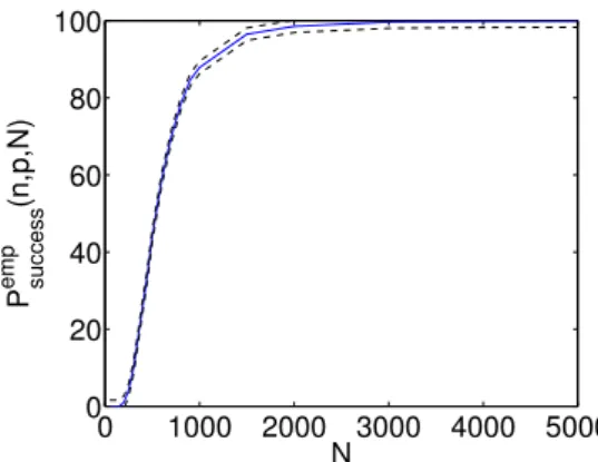
0 1000 2000 3000 4000 5000 0
20 40 60 80 100
N P successemp (n,p,N)
Figure 1: Probability of success (in %) estimated forn= 4 andp= 10 by (7) overm= 10000 samples (plain line) with the error bounds given by (8) atδ= 1% (dashed lines).
modeλi in {1, . . . , n} and with a zero-mean Gaussian noiseei of standard deviationσe= 0.2. The initial- izationwof Algorithm 1 follows a uniform distribution in the rather large interval [−100,100]np, assuming no prior knowledge on the true parameter values.
Section 4.1 below analyzes the influence of the size of the data sets, N, on the probability of success under these conditions, while Section 4.2 further studies the validity of the results for other noise levels.
Finally, Section 4.3 will emphasize the effect of the constraints on the regressors implied by a SARX system.
4.1. Influence of the number of data
Consider the following set of experiments which aim at highlighting the relationship between the number of data and the difficulty of the problem measured through the probability of success of the simplek-LinReg algorithm. For each setting, defined by the triplet of problem dimensions (n, p, N), we generatem= 10000 training sets ofN points, {(xi, yi)}Ni=1, with the equationyi=θTλixi+ei,i= 1, . . . , N, whereθ,xi,λi,ei
are realizations of the corresponding random variables drawn according to the distributions defined above.
For each data set, we apply Algorithm 1 with a random initializationwk and compute the estimate (7) of the probability of success. More precisely, we setǫ= 10−9, which means that an initialization must lead to a value of the cost function (1) very close to the global optimum in order to be considered as successful.
In fact, the analysis considers a slight modification to Algorithm 1, in which the returned value of the objective function, F(wk∗), is arbitrarily set to F(wk∗) = +∞ for problematic cases discussed in Sect. 3 and where, at some iterationtand for some mode j,|{i : λti =j}|< p. More generally, note that, inRp, any set ofp−1 points can be fitted by a single linear model. Therefore, forN ≤n(p−1), there are trivial solutions that minimize the costF(w), but do not correspond to solutions of the modeling problem withn submodels. The modification to Algorithm 1 ensures that such cases are considered as failures throughout the analysis.
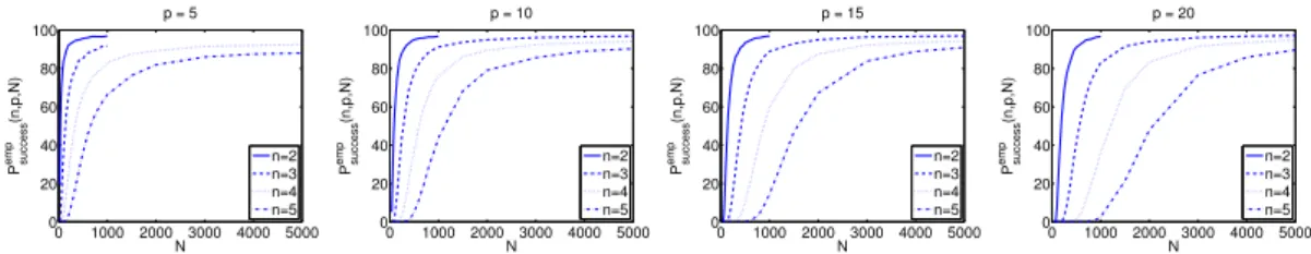
Figure 1 shows a typical curve of the influence of the number of data on the quality of the solution returned by k-LinReg in terms of the quantity (7). The probabilistic bounds within which the true probability of success lies are also plotted and we see that they are very tight. The curves obtained in various settings are reported in Figure 2. These plots of (7) indicate that using more data increases the probability of success, so that the cost function (1) seems to have fewer local minima for largeN than for smallN.
Remark 4. Most approaches that aim at globally solving Problem 1 have difficulties to handle large data sets. This is often related to an increase of the number of optimization variables, which may lead to a prohibitive computational burden. However, this does not necessarily means that the corresponding nonconvex optimization problem is more difficult to solve in terms of the number of local minima or the relative size of their basin of attraction compared with the one of the global optimum. Indeed, the results above provide evidence in favor of the opposite statement: the probability of success of the local optimization Algorithm 1 monotonically increases with the number of data.
0 1000 2000 3000 4000 5000 0
20 40 60 80 100
N Psuccessemp(n,p,N)
p = 5
n=2 n=3 n=4 n=5
0 1000 2000 3000 4000 5000 0
20 40 60 80 100
N Psuccessemp(n,p,N)
p = 10
n=2 n=3 n=4 n=5
0 1000 2000 3000 4000 5000 0
20 40 60 80 100
N Psuccessemp(n,p,N)
p = 15
n=2 n=3 n=4 n=5
0 1000 2000 3000 4000 5000 0
20 40 60 80 100
N Psuccessemp(n,p,N)
p = 20
n=2 n=3 n=4 n=5
0 1000 2000 3000 4000 5000 0
20 40 60 80 100
N Psuccessemp(n,p,N)
p = 50
n=2 n=3 n=4
Figure 2: Estimates of the probability of success,Psuccessemp (n, p, N), versus the number of dataN. Each plot corresponds to a different dimensionpand each curve corresponds to a different number of modesn.
0 1 2 3 4
0 20 40 60 80 100
σe Psuccess
emp(n,p,N)
p = 5
n=2 n=3 n=4
0 1 2 3 4
0 20 40 60 80 100
σe Psuccess
emp(n,p,N)
p = 10
n=2 n=3 n=4
0 1 2 3 4
0 20 40 60 80 100
σe Psuccessemp(n,p,N)
p = 15
n=2 n=3 n=4
0 1 2 3 4
0 20 40 60 80 100
σe Psuccessemp(n,p,N)
p = 20
n=2 n=3 n=4
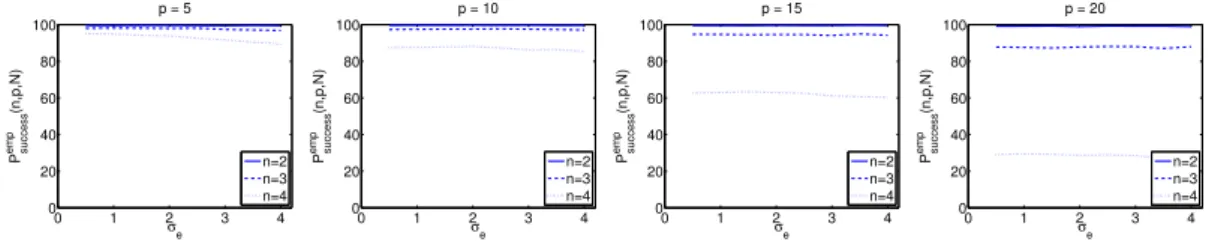
Figure 3: Estimates of the probability of success (in %) versus the noise levelσe for different settings (n, p).
4.2. Influence of the noise level
The analysis in the previous section holds for fixed distributions of the random variables w,θ,X,λ,e, and in particular for the chosen noise level implemented by the standard deviation, σe, of the Gaussian distribution of e. Here, we evaluate the influence of this noise level on the estimates of the probability of success.
Experiments are conducted as in the previous subsection, except for the training set size, N, which is fixed to 1000 and the noise level,σe, which now varies over a grid of the interval [0.5,4.0] (corresponding to a range of about 20 dB in terms of signal-to-noise ratio and reasonable values within which the submodels can be distinguished). This means that for each value of σe on this grid, 10000 samples of the random variables are drawn to compute the estimate of the probability of success via the application of Algorithm 1 and (6)–(7). These experiments are repeated for different problem dimensions (n, p) and the results are plotted in Figure 3. Note that, here, the aim is not to evaluate the range of noise levels that thek-LinReg algorithm can deal with, but instead to determine whether the curves of Figure 2 are sensitive to the noise level.
These results show that the noise level has little influence on the performance of the algorithm. Recall that here, the performance of the algorithm is evaluated as its ability to reach a value of the cost function sufficiently close to the global minimum. Of course, once a solution close to the global one has been found, the noise level influences the accuracy of the parameter estimation, as for any regression algorithm. However, these experiments support the idea that the noise level does not directly determines the level of difficulty of a switched regression problem, which rather lies in the ability of an algorithm to discriminate between the modes. It will therefore be omitted from the predictive model discussed in Section 5 which will focus on the influential parametersnandp.
4.3. Influence of the SARX system structure
This section reproduces the analysis of Sect. 4.1 for SARX system identification instead of switched regression, i.e., for a regression vectorxi= [yi−1, . . . , yi−ny, ui−na, . . . , ui−nb]T, constrained to a manifold of Rp. More precisely,Xis now a deterministic function of the random variablesθ,x0(the initial conditions), u(the input sequence), λande. The probability is now defined overx0,u,λ,einstead ofX,λ,eand with uniform distributions forx0 andu. In addition, for a givenp, we uniformly draw ny in {1, . . . , p−1} and set na = 0, nb =p−ny. Thus, we uniformly sample identification problems with various system orders.
We use a simple rejection method to discard unbounded trajectories without particular assumptions on the
0 1000 2000 3000 4000 5000 0
20 40 60 80 100
N Psuccessemp(n,p,N)
p = 5
n=2 n=3 n=4 n=5
0 1000 2000 3000 4000 5000 0
20 40 60 80 100
N Psuccessemp(n,p,N)
p = 10
n=2 n=3 n=4 n=5
0 1000 2000 3000 4000 5000 0
20 40 60 80 100
N Psuccessemp(n,p,N)
p = 15
n=2 n=3 n=4 n=5
0 1000 2000 3000 4000 5000 0
20 40 60 80 100
N Psuccessemp(n,p,N)
p = 20
n=2 n=3 n=4 n=5
Figure 4: Same curves as in Figure 2, but for SARX system identification.
system whose parametersθremain uniformly distributed in [−1,1]np(depending on the switching sequence, unstable subsystems can lead to stable trajectories and vice versa).
The results are plotted in Fig. 4 and confirm the general tendency of the probability of success with respect to N. However, these results also show that the constraints on the regression vector increase the difficulty of the problem. In particular, both the rate of increase of the probability of success and its maximal value obtained for largeN are smaller than in the unconstrained case reported in Fig. 2.
5. Modeling the probability of success
The following presents the estimation of a model of the probability of success based on the measurements of this quantity derived in the previous section. The aim of this model is to provide a simple means to set the number of restarts fork-LinReg (Section 5.2) and an indication on the number of data with which we can expectk-LinReg to be successful on a particular task (Section 5.3).
More precisely, we are interested in obtaining these numbers from general parameters of a given problem instance summarized by the triplet (n, p, N). In order to fulfill this goal, we require an estimate of the probability of success ofk-LinReg for any given triplet of problem dimensions (n, p, N). Since estimating this probability as in Section 4 for all possible triplets would clearly be intractable, we resort to a modeling approach. Thus, the aim is to estimate a model that can predict with sufficient accuracy the probability Psuccess(n, p, N, ε). Irrespective of the quantity of interest, the classical approach to modeling involves several steps. First, we need to choose a particular model structure. This structure can either be parametric and based on general assumptions or nonparametric as in black-box models. Here, we consider the parametric approach and choose a particular model structure from a set of assumptions. Then, the parameters of this model are estimated from data. Here, the data consist in the estimates of the probability of success obtained in Section 4 for a finite set of triplets (n, p, N). Therefore, in the following, these estimates, Psuccessemp (n, p, N, ε), are interpreted as noisy measurements of the quantity of interest, Psuccess, from which the model can be determined.
This section and the followings are based on the measurements obtained in Sect. 4 with a fixed and small value of the threshold ε= 10−9. Therefore, in the remaining of the paper we will simply use the notation Psuccess(n, p, N) to refer toPsuccess(n, p, N, ε) for this specific value of ε.
The choice of structure for the proposed model relies on the following assumptions.
• The probability of success should be zero when N is too small. Obviously, without sufficient data, accurate estimation of the parameters w is hopeless. In particular, we aim at the estimation of all parameter vectors, {wj}nj=1, and therefore consider that solutions leading to a low error with fewer submodels as inaccurate. More precisely, this is implemented in the data by the modification of Algorithm 1 discussed in Sect. 3 and which returns an infinite error value in such cases.
• The probability of success monotonically increases with N. This assumption is clearly supported by the observations of Section 4. It is also in line with common results in learning and estimation theory, where better estimates are obtained with more data. However, the validity of such assumptions in the context of switched regression was not obvious, since these results usually apply to local algorithms under the condition that the initialization is in the vicinity of the global minimizer (or that the problem is convex).
1 2 3 4 5 6 0.6
0.8 1
n
K
1 2 3 4 5 6
0.6 0.8 1
n
K
0 200 400 600 800
0 1000 2000 3000
2n p
τ
0 200 400 600 800
0 1000 2000
2n p
τ
0 200 400 600 800
0 1000 2000
2n p
T
0 200 400 600 800
0 500 1000 1500
2n p
T
Figure 5: Parameters of the model (9) as obtained from the average curves in Fig. 2 (blue ’+’), the ones in Fig. 4 (black
’◦’) and from the proposed formulas (13)–(18) in a switched regression (top row) or SARX system identification (bottom row) setting.
• The probability of success converges, when N goes to infinity, to a value smaller than one. This assumption reflects the fact that the size of the data set cannot alleviate all difficulties, in particular regarding the issue of local minima. Note that this is an issue specific to the switched regression setting, whereas classical regression algorithms can compute consistent estimates. In switched regression, consistency of an estimator formulated as the solution to a nonconvex optimization problem does not imply the computability of consistent estimates.
• The probability of success should be a decreasing function of bothnandp. This assumption reflects the increasing difficulty of the problem with respect to its dimensions. In particular, with more submodels (largern), more local minima can be generated, while increasing the dimensionpincreases the range of possible initializations and thus decreases the probability of drawing an initialization in the vicinity of the global optimum.
Following these assumptions, we model the probability of success,Psuccess(n, p, N), by the unitary step response of a first order dynamical system with delay, where the number of data N plays the role of the time variable, i.e.,
Pbsuccess(n, p, N) =
K(n, p)
1−exp
−(N−τ(n, p)) T(n, p)
, ifN > τ(n, p)
0, otherwise,
(9) and where the dimensionsnandpinfluence the parameters. In particular,K(n, p) is the “gain”, τ(n, p) is the “time-delay” andT(n, p) is the “time-constant”. Such models are used in Bro¨ıda’s identification method [19], in which the constantsK,τ andT are estimated on the basis of curves as the ones in Figures 2 and 4.
This estimation relies on the following formulas:
K(n, p) = lim
N→+∞Psuccess(n, p, N) = sup
N
Psuccess(n, p, N), (10)
τ(n, p) = 2.8N1−1.8N2, (11)
T(n, p) = 5.5(N2−N1), (12)
whereN1 andN2 are the numbers of data (originally, the “times”) at Psuccess(n, p, N) = 0.28K(n, p) and Psuccess(n, p, N) = 0.40K(n, p), respectively. We use linear interpolation to determine N1 and N2 more precisely from the curves in Fig. 2 and 4 and obtain estimates of the constants K, τ and T for different numbers of modesnand dimensionsp.
As shown by Figure 5, these constants can be approximated by the following functions ofnandp:
K(n, p) = 0.99, (13)
τ(n, p) = 0.2 (2np)1.4, (14)
T(n, p) = 2.22×2np, (15)
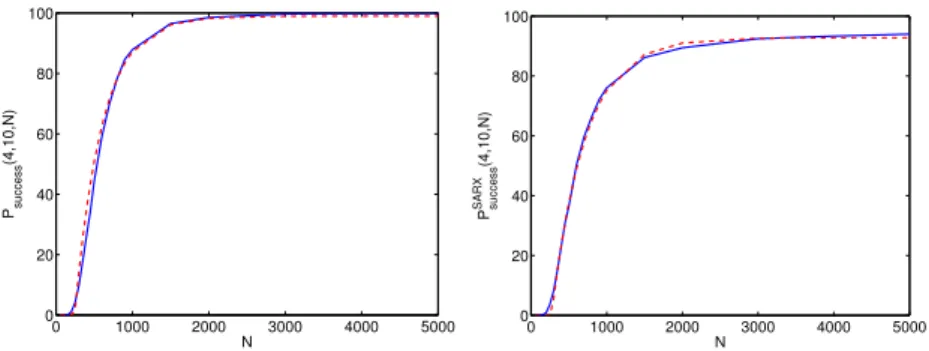
0 1000 2000 3000 4000 5000 0
20 40 60 80 100
N Psuccess(4,10,N)
0 1000 2000 3000 4000 5000
0 20 40 60 80 100
N PsuccessSARX(4,10,N)
Figure 6: Empirical estimates of the probability of success (solid line) and values predicted by the model (7) (dash line) for switched regression (left) and SARX system identification (right). These curves are obtained withn= 4 andp= 10.
for switched regression, while the following approximations are suitable for SARX system identification:
KSARX(n, p) = 1.02−0.023n, (16)
τSARX(n, p) = 1.93×2np−37, (17)
TSARX(n, p) = 52p
2np−220. (18)
The coefficients in these equations are the least squares estimates of the generic parametersaandb in the linear regressions K(n, p) = an+b, ˜τ =a˜z+b and T(n, p) =az+b, where z = 2np, ˜τ = logτ(n, p) and
˜
z= logz. For SARX systems, the relationships givingτSARX andTSARX are modified asτSARX(n, p) = az+bandTSARX(n, p) =a√
z+b.
Finally, the model of the probability of success is given either by Pbsuccess(n, p, N) =
0.99
1−exp
−(N−0.2(2np)1.4)
2.22×2np
, ifN >0.2 (2np)1.4
0, otherwise,
(19)
in a regression setting or by, PbsuccessSARX(n, p, N) =
((1.02−0.023n)
1−exp
−(N−1.93×2np−37) 52√2np−220
, ifN >1.93×2np−37
0, otherwise, (20)
for SARX system identification. The output of these models is very close to the empirical average of Psuccess(n, p, N) as illustrated for n = 4 and p = 10 by Figure 6. The mean absolute error, 1/|T |P
(n,p,N)∈T |Psuccess(n, p, N)−Pbsuccess(n, p, N)|, over the set of triplets,T, used for their estimation, is 0.048 for Pbsuccess(n, p, N) and 0.102 forPbsuccessSARX(n, p, N).
5.1. Estimation of the generalization ability of the model via cross-validation
The generalization error of the models (19)-(20) reflects their ability to accurately predict the probability of success for triplets (n, p, N) not inT, i.e., for previously unseen test cases. This generalization error can be estimated from the data through a classical cross-validation procedure (see, e.g., [20]), which iterates over KCV subsets of the data. At each iteration, the model is estimated fromKCV −1 subsets and tested on the remaining subset. The average error thus obtained yields the cross-validation estimate of the generalization error.
Since the computation of each value of the constantsK, τ, T (each point in Fig. 5) rely on an entire curve with respect toN, we split the data with respect tonand p: all data in a subset correspond to a curve in Fig. 2 or 4 for fixed (n, p). Then, at iterationk, the models (19)-(20) are estimated without the data for the
setting (nk, pk) and the sum of absolute errors,|Psuccess(nk, pk, N)−Pbsuccess(nk, pk, N)|, is computed over allN.
Applying this procedure leads to a cross-validation estimate of the mean absolute error of 0.050 for switched regression and 0.105 for SARX system identification. Though the model is less accurate for SARX systems, its error remains reasonable for practical purposes such as the automatic tuning of the number of restarts fork-LinReg, as proposed next.
5.2. Computing the number of restarts for k-LinReg
Consider now the algorithm restartedrtimes with initializations that are independently and identically drawn from a uniform distribution. The probability of drawing a successful initialization for a particular problem instance, i.e., for givenθ,X,λande, is the conditional probability of successPcond(θ,X,λ,e) = Pw|θ,X,λ,e(F(w∗)−F(θ) ≤10−9) and the probability of not drawing a successful initialization in any of the restarts is
Pf ail(r) = Yr k=1
(1−Pcond(θ,X,λ,e)) = (1−Pcond(θ,X,λ,e))r. (21) To set the number of restarts, we consider the average probability of drawing a successful initialization, where the average is taken over all problem instances, i.e., we consider the expected value of the conditional probability of success Pcond(θ,X,λ,e). This expectation corresponds to the joint probability of success, Psuccess(n, p, N) =Pw,θ,X,λ,e(F(w∗)−F(θ)≤10−9), since
Psuccess(n, p, N) =Ew,θ,X,λ,e[I(F(w∗)−F(θ)≤10−9)]
=Eθ,X,λ,eEw|θ,X,λ,e[I(F(w∗)−F(θ)≤10−9)|θ,X,λ,e]
=Eθ,X,λ,e[Pcond(θ,X,λ,e)].
Considering the mean conditional probability, i.e., replacingPcond(θ,X,λ,e) by Psuccess(n, p, N) in (21), leads to a trade-off between optimistic estimates for difficult problems and pessimistic ones for easier prob- lems. This trade-off allows us to build an algorithm that is both computationally efficient and sufficiently successful on average. This algorithm relies on the following estimate of the probability of failure:
Pbf ail(r) = (1−Pbsuccess(n, p, N))r.
Then, the number of restarts r∗ required to obtain a given maximal probability of failure Pf∗ such that Pbf ail(r)≤Pf∗, is computed as
r∗= min
r∈N∗ r, s.t. r≥ logPf∗ log
1−Pbsuccess(n, p, N), (22)
wherePbsuccess(n, p, N) is given by (19) or (20).
In practice, the bound in (22) can be used as a stopping criterion on the restarts of the algorithm once the value of the hyperparameterPf∗ has been set. This leads to Algorithm 2, which can easily be cast into a parallel form by executing the line in italic multiple times in separate working threads.
The internal box bounds on the initialization vectors, [w,w], can be used to include prior knowledge on the values of the parameters, but they can also be set to quite large intervals in practice. Note that these bounds do not constrain the solution of the algorithm beyond the initialization, so thatwbest∈/ [w,w] can be observed.
5.3. Estimating the sample complexity
We define the sample complexity ofk-LinReg at levelγas the minimal size of the training sample,N(γ), leading to
Psuccess(n, p, N)≥γ.
Algorithm 2k-LinReg with multiple restarts
Require: the data set (X,y)∈RN×p×RN, the number of modes nand the probability of failurePf∗. InitializeFbest= +∞and k= 0.
ComputeK, τ,T as in (13)-(15) or (16)-(18).
Setr∗according to (22).
repeat k←k+ 1.
Draw a random vectorw uniformly in [w,w]⊂Rnp.
Apply Algorithm 1 initialized atw to get the pair (F(w∗),w∗).
if F(w∗)< Fbest then
Update the best local minimumFbest←F(w∗) and minimizerwbest←w∗. end if
until k≥r∗.
return Fbest andwbest.
After substituting the modelPbsuccess(n, p, N) forPsuccess(n, p, N) in the above, this sample complexity can be estimated by using (9) as
Nb(γ)≥τ(n, p)−T(n, p) log
1− γ
K(n, p)
, ifγ < K(n, p),
Nb(γ) = +∞, otherwise.
(23) In a given setting with n and pfixed, this can provide an indicative lower bound on the number of data required to solve the problem with probabilityγby a single run ofk-LinReg. The caseNb(γ) = +∞reflects the impossibility to reach the probability γ, which may occur for unreasonable values of γ > 0.99 or for SARX systems with a very large number of modesn.
However, note that (23) is mostly of practical use, since its analytical form depends on the particular choice of structure for (9).
6. Numerical experiments
This section is dedicated to the assessment of the model of the probability of success (19) as a means to tune the number of restarts on one hand and of thek-LinReg algorithm as an efficient method for switched linear regression on the other hand. Its time efficiency is studied in Sec. 6.1 and 6.2 with respect to the number of data and the problem dimensions, respectively. Section 6.3 analyses the ability of the method to reach global optimality, while Sec. 6.4 is dedicated to its application to hybrid dynamical systems.
Thek-LinReg method is compared with the approach of [10], which directly attempts to globally optimize (1) with the Multilevel Coordinate Search (MCS) algorithm [21] and which we label ME-MCS. The second version of this approach, based on a smooth product of error terms, is also included in the comparison and labeled PE-MCS. We also consider the algebraic approach [2], which can deal efficiently with noiseless data, and the recent sparse optimization-based method [11]. The application of the latter is slightly different as it requires to set a threshold on the modeling error instead of the number of modes. The comparison with this approach will therefore only be conducted on the example taken from [11].
Three evaluation criteria are considered: the computing time, the mean squared error (MSE) computed by the cost function (1), and the normalized mean squared error on the parameters (NMSE) evaluated against the true parameter values{θj} as
NMSE = 1 n
Xn j=1
kθj−wjk22
kθjk22
, (24)
for the set of estimated parameter vectors {wj} ordered such that the NMSE is minimum. All numbers reported in the Tables and points in the plots are averages computed over 100 random problems generated
with a different set of parameters{θj}, except for the examples in Sect. 6.4 where the parameters are fixed and the averages are taken over 100 trials with different noise sequences.
For indicative purposes, a reference model is also included in the experiments and corresponds to the model obtained by applyingnindependent least-squares estimators to the data classified on the basis of the true mode (which is unknown to the other methods).
Except when mentioned otherwise, k-LinReg refers to Algorithm 2, which is stopped after completing the number of restartsr∗ given by (22) with a maximal probability of failurePf∗= 0.1% and with the model (19), or (20) for the examples of Sect. 6.4. The bounds on the initialization are always set tow=−100·1np
andw = 100·1np. The web page at http://www.loria.fr/~lauer/klinreg/provides open source code fork-LinReg in addition to all the scripts used in the following experiments.
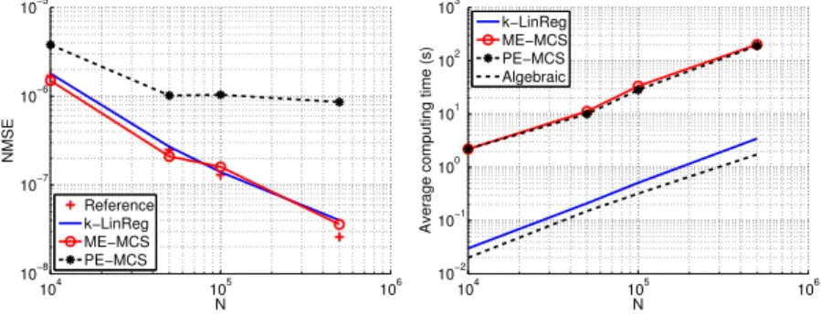
6.1. Large data sets in low dimension
The performance of the methods on large data sets is evaluated through a set of low-dimensional problems with n = 2 and p = 3, in a similar setting as in [10]. The N data are generated by yi = θTλixi +vi, with uniformly distributed random regression vectorsxi∈[−5,5]p, a random switching sequence{λi} and additive zero-mean Gaussian noisevi of standard deviationσv = 0.2. The goal is to recover the set of true parameters{θj}randomly drawn from a uniform distribution in the interval [−2,2]p in each experiment.
104 105 106
10−8 10−7 10−6 10−5
NMSE
N Reference k−LinReg ME−MCS PE−MCS
104 105 106
10−2 10−1 100 101 102 103
Average computing time (s)
N k−LinReg ME−MCS PE−MCS Algebraic
Figure 7: Average NMSE (left) and computing time (right) over 100 trials versus the number of dataN(plots in log-log scale).
Figure 7 shows the resulting NMSE and computing times of k-LinReg, ME-MCS and PE-MCS, as averaged over 100 experiments for different numbers of data N. The computing time of the algebraic method, considered as the fastest method for such problems, is also shown for indicative purposes though this method cannot handle such a noise level (times are obtained by applying it to noiseless data). All computing times are given with respect to Matlab implementations of the methods running on a laptop with 2 CPU cores at 2.4 Ghz. The k-LinReg algorithm is much faster than the general purpose MCS algorithm and almost as fast as the algebraic method, while still leading to very accurate estimates of the parameters. In particular, the average NMSE ofk-LinReg is similar to the ones obtained by the reference model and the ME-MCS. However, the ME-MCS algorithm fails to find a relevant model (with NMSE
<1) in a number of cases which are not taken into account in its average NMSE. Note that thek-LinReg estimates are found with only two random initializations since (22) leads tor∗= 2 in this setting.
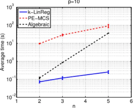
6.2. High dimensions
Figure 8 shows the average computing times over 100 random experiments of thek-LinReg, the PE-MCS and the algebraic methods versus the dimensionp. Data sets ofN = 10 000 points are generated as in the previous subsection with a noise standard deviation ofσv = 0.1, except for the algebraic method which is applied to noiseless data in order to produce consistent results. The reported numbers reflect the computing times of Matlab implementations of the three methods as obtained on a computer with 8 cores running at 2.53 GHz. For low dimensions, i.e.,p≤5, the k-LinReg algorithm is slightly slower than the algebraic method, with however computing times that remain below 1 second. For high dimensions, p ≥ 50, the