The theoretical rationale for such kernels is further founded on the use of reproducing kernel Hilbert spaces in which the measures are embedded, together with elements of convex analysis and descriptors of the measures used in statistics and information theory, such as variance and entropy. One of the most interesting of these shifts is undoubtedly the increasing variety of data structures we now face.
Nuts and Bolts of Kernel Methods
The Multiple Facets of Kernels in Machine Learning 4
1.3) The first problem is called kernel PCA in the seminal work of Scholkopf et al. 1998) and amounts to a simple decomposition of the kernel matrix KX with singular values. However, the subject of this thesis does not concern this part of the kernel machinery.
Blending Discriminative and Generative Approaches with Kernels 15
Nonparametric Kernels on Measures
When this knowledge is a kernel in the components, "kernelized" estimates of the kernels over the measures can be computed. In the first paper, the authors review a large family of models for which the family of Bhattacharrya kernels can be calculated directly.
Contribution of this Thesis
- A String Kernel Inspired by Universal Coding
- Semigroup Kernels on Measures
- Spectral Semigroup Kernels on Measures
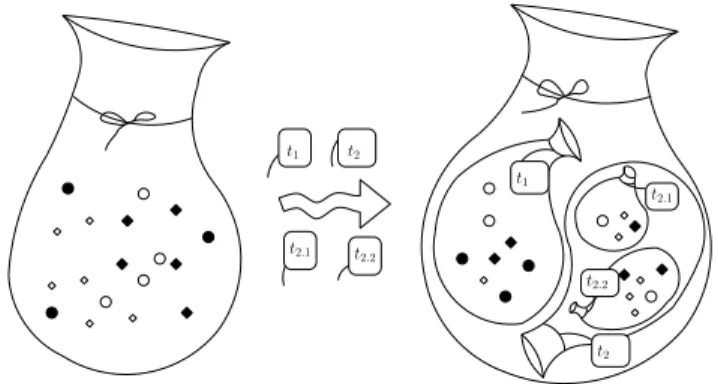
- A Multiresolution Framework for Nested Measures . 22
The main inspiration behind the context tree kernel is the algorithmic efficiency of the context tree weighting (CTW) algorithm presented by (Willems et al., 1995) and further studied in (Catoni, 2004). A more complete overview of the application of kernel methods in computational biology is presented in (Sch¨olkopf et al., 2004).
Probabilistic Models and Mutual Information Kernels
We present further interpretations of the context tree kernel computation, as well as links to universal encoding in Section 2.5. We consider these limitations in light of the solution proposed by the CTW algorithm in the context of universal encryption, to define an appropriate set of models and prior distributions below.
A Mutual Information Kernel Based on Context-Tree Models . 28
Context-Tree Models
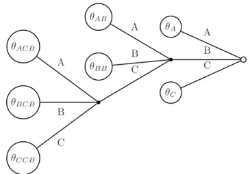
We write L(D) for the length of the longest word in D and FD for the set c.s.d D that satisfies L(D)≤D. Conversely, a context-tree distribution D can be easily expressed as a Markov chain by assigning the transition parameters θs to all the contexts in ED that allow s as their unique suffix in D .
Prior Distributions on Context-Tree Models
For a given treeD, we now define a prior for the family of multinomial parameters ΘD= (Σd)D, which fully characterizes a context-tree distribution based on a dictionary of suffixesD. The parameter β encapsulates whatever prior belief we have about the division of the alphabet.
Triple Mixture Context-Tree Kernel
Kernel Implementation
Defining Counters
For contexts present in the stringX, i.e. words such as datρm(X)>0, the empirical behavior of transitions can be estimated as.
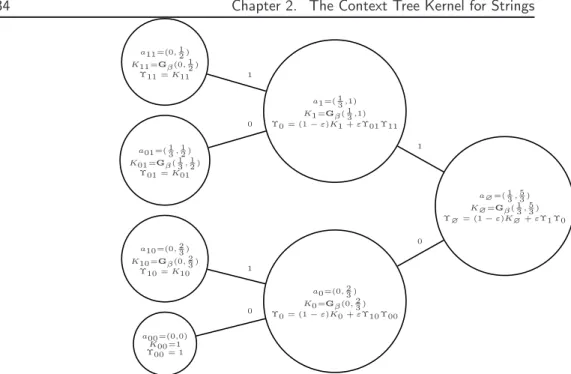
Recursive Computation of the Triple Mixture
As previously recalled, computing the counters has a linear cost in time and memory with respect to D(NX+NY). As a final result, the computation of the kernel is linear in time and space with respect to D(NX+NY).
Source Coding and Compression Interpretation
These coordinates, whose information is equivalent to that contained in the spectrum of the sequence, can be used to compute the probability of a specific context-tree distribution (D, θ) on such a set by deriving {(ρs,θˆs), s ∈ D} recursively, as in the previous calculation. The choice of a compression algorithm (namely a selection of priors) defines the shape of the function rπ on the entire space of counters, and the similarity between two sequences is measured through the difference between three evaluations of rπ, first taken at the two points taken apart and then at their average, which is directly related to the convexity of rπ.
Experiments
Protein Domain Homology Detection Benchmark
The entire family of context tree kernels is therefore defined by a prior belief about the behavior of sequence counters (set by a selection of specific priors), which is first applied to the sequences individually. This point of view can also bring forth a geometrical perspective on the actual calculation being performed.
Parameter Tuning and Comparison with Alternative
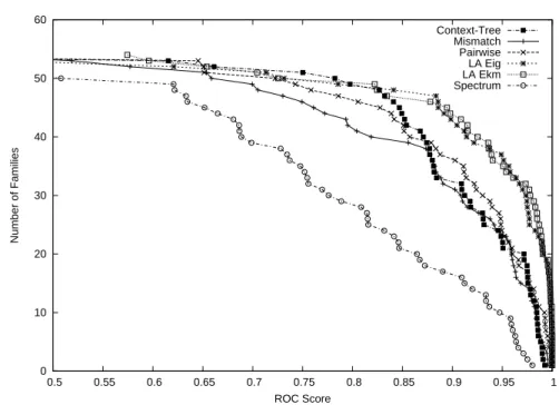
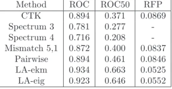
40 Chapter 2. Context Tree Kernel for Strings fournier20.compand dist20.comp) which can be downloaded from a Dirichlet mixture repository13. We also report the results of the spectrum kernel (Leslie et al., 2002) with depths 3 and 4 and show that, based on the same information (D-grams), the context extractor clearly outperforms the latter.
Mean Performances and Curves
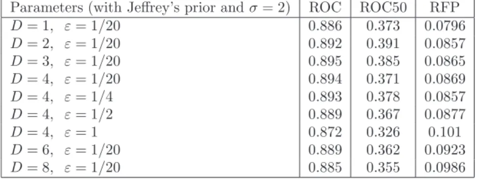
As can be easily deduced from the previous figure, the context tree kernel clearly outperforms the spectrum kernel while using exactly the same information. Finally, in Table 2.2 we present some results for significant settings of the context tree kernels using Jeffrey's prior.
Closing remarks
In this case, when no blend is performed on the model class, the computation of the context tree is similar to the simpler computation performed by the spectrum kernel. Note also that good performance is obtained when the context tree uses only contexts of length 1 (namely Markov chains of depth 1), indicating that the models should be selected for feature extraction rather than sequence modeling, a hint further supported by the fact , that long trees do not perform very well despite their better ability to absorb more knowledge about string transitions.
Introduction
In the case of a kernel based on the spectrum of the variance matrix, we show how. Finally, Section 5.4 contains an empirical evaluation of the proposed kernels on a comparative handwritten digit classification experiment.
Notations and Framework
Measures on Basic Components
Using the general theory of semigroup kernels, we establish an integral representation of such kernels and study the semicharacters involved in this representation. Through regularization procedures, practical applications of such kernels to molecular benchmarks are presented in Section 3.4, and the approach is further extended by kernelizing the IGV via an a priori kernel defined itself on the space of components in Section 3.5.
Semigroups and Sets of Points
First, it performs the union of the supports; second, the sum of such molecular measures also adds the weights of the points common to both measures, with a possible renormalization on these weights. However, two important features of the original list are lost in this mapping: the order of its elements and the original frequency of each element in the list as a weighted singleton.
The Entropy and Inverse Generalized Variance Kernels
Entropy Kernel
The comparison between the two densities f, f′ in that case is performed by integrating pointwise the squared distance between the two densities d2(f(x), f′(x)) over X, using the forda distance chosen between a family of appropriate metric in R+ to ensure that the final value is independent of the dominant measure. While both e−h and−J can be used in practice for non-normalized measures, we more clearly name kh = e−J the entropy kernel because it actually quantifies when f and f′ are normalized (ie, such that |f| = |f′| = 1) is the difference of the mean entropy of off andf' from the entropy of their mean.
Inverse Generalized Variance Kernel
Note that only - it is a strictly semigroup kernel, since -J involves a normalized sum (via division by 2) which is not associative. The subset of absolutely continuous probability measures on (X, ν) with finite entropy, namely f ∈M+h(X), s.t.|f|= 1 is not a semigroup since it is not closed by addition, but still we can we determine the restriction of J and thus kh on it to obtain a p.d.
Semigroup Kernels on Molecular Measures
Entropy Kernel on Smoothed Estimates
Regularized Inverse Generalized Variance of Molec-
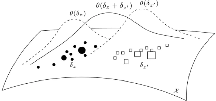
Given two objects z, z′ and their respective molecular masses δz and δz′, calculating the IGV for two such objects requires in practice an acceptable basis of δz+δ2z′ as seen in Theorem 3.6. This acceptable basis can be chosen to be of the support cardinality of the mixture of δz and δz′, or alternatively to be.
Inverse Generalized Variance on the RKHS associated with a
The weight matrices ∆γ and ∆φ(γ) are identical, and we further have K˜γ = ˜Kφ(γ) by the reproducing property, where ˜K is defined by the dot product of the Euclidean space Υ induced by κ. As observed in the experimental section, the kernelized version of the IGV is more likely to be successful in solving practical tasks since it incorporates meaningful information about the components.
Integral Representation of p.d. Functions on a Set of Measures . 61
In both cases, if the integral representation exists, then there is uniqueness of the measureω inM+(S∗). When using unbounded functions (as is the case when expectation or second-order moments of measures are used) the continuity of the integral is left undetermined to our knowledge, even when its existence is assured.
Experiments on images of the MNIST database
Linear IGV Kernel
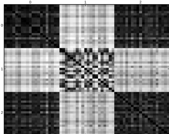
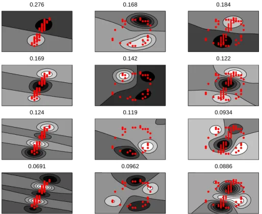
The linear IGV kernel as described in Section 3.3.2 is equivalent to using the linear kernelκ((x1, y1),(x2, y2)) =x1x2+y1y2 on a non-regularized version of the kernelized IGV. Normalized Gram matrix calculated with the linear IGV kernel of twenty images of “0”, “1” and “2” shown in that order.
Kernelized IGV
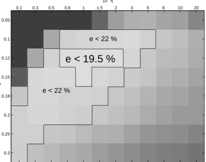
The two parameters are closely related, as the value of σ controls the range of typical eigenvalues found in the spectrum of Gram matrices of acceptable bases, while η acts as a scaling parameter for those eigenvalues as can be seen in equation (3.3) . The resulting eigenvalues for ˜K∆ are all very close to 1d, the inverse of the number of points considered.
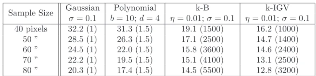
Experiments on the SVM Generalization Error
The results presented in Table 5.1 of the k-IGV kernel show a consistent improvement over all other kernels for this benchmark of 1000 images, under all sampling schemes. Besides a minimal number of points needed to perform sound estimation, the size of submitted samples positively affects the accuracy of the k-IGV kernel.
Closing remarks
We further investigate theoretical properties and characterizations of both half-characters and positive definite functions on targets. First, and when the space of components is set, the representation of an object as a target can be effectively achieved through statistical estimation, to represent and regulate these targets correctly, e.g. the use of uniform Dirichlet priors in Cuturi and Vert (2005) to regularize letter counts or tfidf type frequencies for words (Lafferty and Lebanon, 2005; Joachims, 2002).
Comparing Measures on Arbitrary Spaces through Kernelized
Measure Representations of Objects and Component
When the component space is too small, essential details about the objects are eventually lost. Semigroup spectral functions on the measures Instead of directly adjusting the empirical measures, another direction involves this smoothing step in expressing the kernel itself on the measures, using in this sense a kernel in the component space.
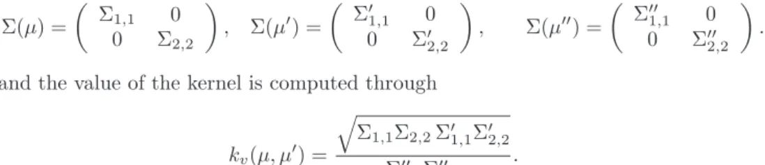
Computing Kernels on Measures through Variance . 80
In Euclidean spaces, variance matrices can be seen as an elementary characteristic of the distribution of a measure. Instead, the approach taken in (Cuturi et al., 2005) is to directly use the second-order moment of the mean of the two measures instead of taking the measures separately.
Semigroup Spectral Functions of Measures
- An Extended Framework for Semigroup Kernels
- Characteristic Functions and s.s.p.d. Kernels
- A Few Examples of Semigroup Spectral Functions . 85
- The Trace Kernel on Molecular Measures
- Practical Formulations for the Trace Kernel
Furthermore, while the square of the Hilbert norm of a difference is always negative definite (Berg et al., 1984, Section 3.3) in both arguments, the reverse is not true in general. Let us consider another example with Wishart density on Σ+n, that is, density with measure Lebesgueν of type.
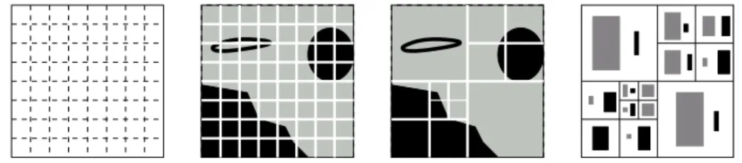
Multiresolution Kernels
Local Similarities Between Measures Conditioned by
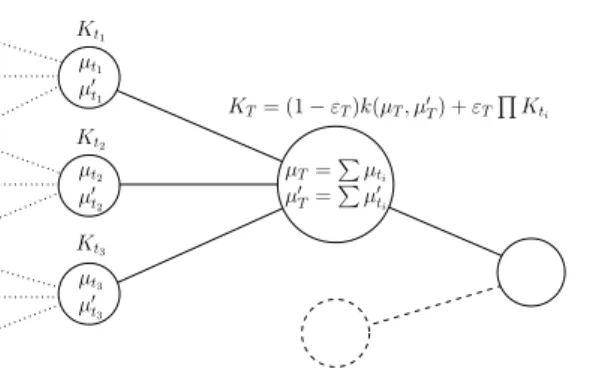
If, on the other hand, the events are assumed to be the same, then they can be considered a unique event{s} ∪ {t} and result in the kernel. The preceding formula can be extended to model kernels indexed on a set T ⊂ T of similar events, through.
Resolution Specific Kernels
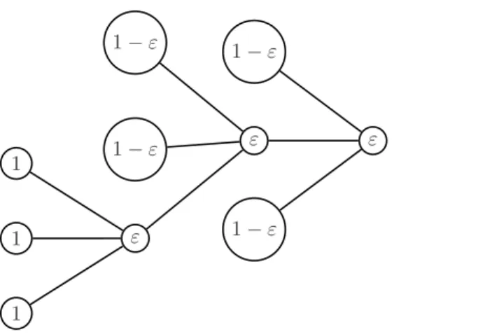
For interpretation purposes only, we may sometimes assume in the following sections that k is an infinitely divisible kernel that can be written as e−ψ, where ψ is a negative definite kernel of M+s(X). To provide a hierarchical content, the family (Pd)Dd=1 is such that any subset present in a partition Pd is included in a (unique by definition of a partition) subset included in the coarser partitionPd−1, and further assume this inclusion to be strict.
Averaging Resolution Specific Kernels
Let's write α, β for the coordinates of the multinomial, where α+β = 1 on the edge of the simplex. In Israil, S., Pevzner, P., and Waterman, M., editors, Proceedings of the Third Annual International Conference on Computational Molecular Biology (RECOMB), pages 15–24, Lyon, France.