HAL Id: hal-03501313
https://hal.inria.fr/hal-03501313
Submitted on 23 Dec 2021
HAL
is a multi-disciplinary open access archive for the deposit and dissemination of sci- entific research documents, whether they are pub- lished or not. The documents may come from teaching and research institutions in France or abroad, or from public or private research centers.
L’archive ouverte pluridisciplinaire
HAL, estdestinée au dépôt et à la diffusion de documents scientifiques de niveau recherche, publiés ou non, émanant des établissements d’enseignement et de recherche français ou étrangers, des laboratoires publics ou privés.
Fault-Tolerant Mapping of Real-Time Parallel Applications under multiple DVFS schemes
Minyu Cui, Angeliki Kritikakou, Lei Mo, Emmanuel Casseau
To cite this version:
Minyu Cui, Angeliki Kritikakou, Lei Mo, Emmanuel Casseau. Fault-Tolerant Mapping of Real-Time Parallel Applications under multiple DVFS schemes. RTAS 2021 - 27th IEEE Real-Time and Em- bedded Technology and Applications Symposium, May 2021, Samos Island, Greece. pp.387-399,
�10.1109/RTAS52030.2021.00038�. �hal-03501313�
(will be inserted by the editor)
Fault-Tolerant Mapping of Real-Time Parallel Applications under multiple DVFS schemes
Minyu Cui, Angeliki Kritikakou, Lei Mo, Emmanuel Casseau
Abstract On multicore platforms, reliable task execution, as well as low en- ergy consumption, are essential. Dynamic Voltage/Frequency Scaling (DVFS) is typically used for energy saving, but with a negative impact on reliability, especially when the frequency is low. Using high frequencies to meet reliabil- ity constraints is not always feasible, while multiple replicas increase energy consumption. To minimize energy consumption, enhancing reliability, with- out violating real-time constraints, we propose an approach that combines distinct reliability enhancement techniques, under task-level, processor-level and system-level DVFS. Our task mapping problem jointly optimizes task allocation, task frequency assignment, and task duplication, under multiple constraints. This is achieved by formulating the task mapping problem as a mixed integer non-linear programming problem and equivalently transforming it into a mixed integer linear programming, that is optimally solved. From the obtained results, the proposed approach achieves better energy consumption and finds solutions, when other approaches fail.
Acknowledgements This work is founded by China Scholarship Council (CSC).
Minyu Cui
Univ Rennes, INRIA, CNRS, IRISA, France, E-mail: minyu.cui@irisa.fr Angeliki Kritikakou
Univ Rennes, INRIA, CNRS, IRISA, France, E-mail: angeliki.kritikakou@irisa.fr Lei Mo
School of Automation, Southeast University, China, E-mail: lmo@seu.edu.cn Emmanuel Casseau
Univ Rennes, INRIA, CNRS, IRISA, France, E-mail: emmanuel.casseau@irisa.fr
1 Introduction
1.1 Context
Hard real-time applications require bothtiming guarantees andreliable execu- tion, i.e., tasks must finish correctly and before their deadlines. To ensure tim- ing guarantees, a safe estimation of the Worst-Case Execution Time (WCET) of tasks is typically used. Nevertheless, the correct execution of tasks is threat- ened by sources that affect hardware platforms, such as radiation and electro- magnetic interference, causing non-persistent transient faults (also known as soft errors). As technology size reduces, platforms become more susceptible to soft errors. Meanwhile, the energy consumption of embedded systems has be- come a crucial factor, especially for systems with a limited energy budget. As a result, adaptive management techniques have been established to maximize energy efficiency [1]. DVFS is a technique that optimizes energy consumption by simultaneously scaling down the processor supply voltage and frequency, during execution. However, DVFS has a significant, negative impact on sys- tem reliability, mainly because of the increased transient fault rates at low supply voltage and frequency levels [2]. Therefore, task mapping techniques must take into account the reliability degradation, energy consumption and execution time in order to make provisions accordingly, especially for real-time applications [3].
1.2 Related work and motivation
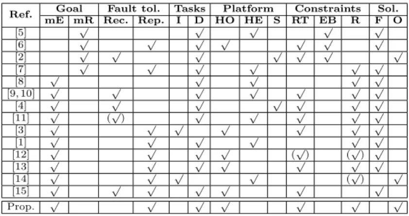
Although both fault tolerance and energy management have been extensively (but often independently) studied, the co-management of system reliability and energy efficiency has been addressed only recently [4]. Table 1 depicts representative State-of-the-Art (SoA) task mapping approaches with DVFS, under Energy Budget (EB), Real-Time (RT) and Reliability (R) constraints, with maximizing system Reliability (mR) or minimizing Energy consumption (mE) goals. Fault tolerance is provided by Recovery tasks (Rec.) or task Repli- cas (Rep.). A task is executed successfully, if at least one replica is executed without faults [3]. Tasks are Independent (I) or Dependent (D). The platform has a Homogeneous (HO), Heterogeneous (HE) or Single (S) processor. Based on the problem formulation and solving method, the solutions are Feasible (F) or Optimal (O).
Regarding reliability maximization, approaches without fault tolerance map only original tasks, e.g., through online heuristics [5]. Approaches with fault- tolerance i) insert a recovery task, always executed with maximum frequency in case of an error [2], ii) map a given number of task replicas [6], and iii) decide the number of replicas during task mapping [7].
Regarding minimizing energy consumption, approaches exist without fault tolerance, e.g., by decomposing the task mapping problem into two sub-problems (satisfying reliability goal and minimizing resource consumption) [8]. To tackle
the negative impacts of DVFS on reliability, existing techniques preserve the original system reliability for all tasks, i.e., the reliability obtained with the maximum platform frequency. Slack is reserved to execute a recovery task (in- dividual [9] or shared [4]) with the maximum frequency. Then, DVFS scales down tasks. If an error is detected, the recovery task is evoked. A longest- task-first heuristic applies DVFS and recovery tasks only to a task subset [10].
However, such approaches usually require high frequencies to satisfy the origi- nal reliability, increasing energy consumption. It is also possible that reliability constraints cannot be satisfied, even with the maximum frequency, leading to empty solution space.
Other approaches compute the required number of replicas to always meet reliability constraints. Heuristics are typically proposed, due to high complex- ity, e.g., a first-fit decreasing heuristic for homogeneous platforms [3] and a list scheduling heuristic for heterogeneous platforms [1]. Hybrid approaches use a given number of replicas and apply task recovery, when an error occurs [13].
However, the increased number of replicas leads to large energy consumption, combined with a negative impact on execution time. When the real-time con- straints are strict, solutions may not exist. To reduce this negative impact, the number of replicas is restricted. In [12], a heuristic decides among single execution, task duplication and task triplication. However, no guarantees are provided on real-time and reliability constraints. In [15], a heuristic determines which tasks to be duplicated, removing the need of a recovery task, without considering any reliability constraint. An Integer Linear Programming (ILP) approach [14] maps independent tasks on a heterogeneous platform to sat- isfy a given percentage of duplicated tasks, under energy budget constraint.
However, the reliability of tasks is not considered.
Table 1: Comparison with representative State-of-the-Art
Ref. Goal Fault tol. Tasks Platform Constraints Sol.
mE mR Rec. Rep. I D HO HE S RT EB R F O
[5] √ √ √ √ √
[6] √ √ √ √ √ √ √
[2] √ √ √ √ √ √ √
[7] √ √ √ √ √ √
[8] √ √ √ √ √
[9, 10] √ √ √ √ √ √ √
[4] √ √ √ √ √ √ √
[11] √
(√
) √ √ √ √ √
[3] √ √ √ √ √ √ √
[1] √ √ √ √ √ √
[12] √ √ √ √
(√
) (√
) √
[13] √ √ √ √ √ √ √
[14] √ √ √ √
(√
) √
[15] √ √ √ √ √ √ √
Prop. √ √ √ √ √ √ √
1.3 Contributions
This work belongs to the last category, extending the SoA by proposing an optimal task mapping approach, which decides between reliable single task ex- ecution and task duplication, under real-time and reliability constraints. The execution of a task is considered safe, when it meets its reliability constraint.
Otherwise, the task requires duplication. As a result, the number of duplicated tasks is reduced, relieving the negative impact on execution time and energy consumption. We focus on the design-time phase, where task mapping and scheduling is performed offline. The goal is to minimize energy consumption, by optimally and concurrently deciding which tasks to be duplicated, the fre- quency per task and the task allocation, under both real-time and reliability constraints. Unlike the majority of SoA techniques, original and duplicated tasks can have different operating frequencies, being more suitable for real- world systems [6]. To achieve that, the task mapping problem is formulated as a Mixed Integer Non-Linear Programming (MINLP), and safely transformed into a Mixed Integer Linear Programming (MILP) problem, in order to be solved optimally. Last, but not least, the proposed approach is extended for three DVFS schemes, typically supported by hardware platforms. To support our contribution, we performed extensive experiments, under different scenar- ios. From the results, the proposed approach can find feasible solutions, when existing replication approaches fail, and consumes less energy, compared to existing reliability-aware approaches.
The rest of the paper is organized as follows. Section 2 introduces the system model. Section 3 presents the formulation of the proposed approaches.
Section 4 presents the evaluation results. Finally, Section 5 concludes this study.
2 System Model
2.1 Task Model
This work considers a real-time application consisting ofN frame-based non- preemptive dependent tasks{τ1, . . . , τN}. The application is represented by a Directed Acyclic Graph (DAG)G(V,E), whereVdenotes the set of tasks and E represents the partial order, corresponding to the precedence constraints among tasks. All the tasks are released at time 0. The ready time of a task is the time instant at which all its predecessors have been completed. Each task τiis defined by its deadlineDiand Worst-Case Execution Cycles (WCEC)Ci. The common period of the tasks is given by the application frame, denoted by H. Hence, the deadline Di cannot be larger than the application frame H, i.e., Di ≤ H. Different functions within an application exhibit distinct vulnerabilities to soft errors, due to variations in the spatial and temporal vulnerabilities of different instructions [12]. Hence, each task τi has its own reliability thresholdRthi .
2.2 Platform Model
A shared-memory multicore platform is used withM homogeneous processors {θ1, . . . , θM}. DVFS is possible at the task (TL-DVFS), processor (PL-DVFS) and system levels (SL-DVFS). Such variants correspond to DVFS-schemes in existing hardware platforms, e.g., clock frequency is controlled per core in Intel-Xeon E5620 and per 8 cores in GreenWaves GAP8. There are L pairs of frequency/voltage levels{(f1, v1), . . . ,(fL, vL)}. Similar to [1, 4, 13], the re- lationship of voltage and frequency is almost linear. Therefore, we use the term frequency scaling to express the simultaneous change of voltage and fre- quency. When task τi is executed with frequency fl, its execution time is ti = Cfi
l. The power consumption is modeled as the sum of static power Plsta and dynamic power Pldyn with the given voltage/frequency level (vl, fl), i.e., Pl = Plsta+Pldyn =Plsta+Cef fv2lfl, where Cef f is the effective switching capacitance [16].
2.3 Processor Fault Model and Reliability
As transient faults have a higher occurrence than permanent faults [8], we focus on transient faults and fault detection is assumed to be done by the hardware.
Our fault model is the one typically used by the SoA, such as [1, 4, 7, 8, 13], i.e., a Poisson distribution with an average fault rate λ(f) at frequency f. Different frequency scalings yield various failure rates. The failure rate per time unit of a processor at frequencyf is given byλ(f) =λ0×10d0
fmax−f fmax−fmin, where fmax = max∀l{fl}, fmin = min∀l{fl}, λ0 is the average failure rate of the processor corresponding tofmax, andd0is a positive constant, indicating the sensitivity of failure rates to voltage scaling [1]. The reliability of a task τi is defined as the probability of executing a task without any fault, based on the exponential model of [17]. Therefore, the reliability of a task with WCEC Ci at frequency fl is ri(fl) = e−ϕi(fl), where ϕi(fl) = λ(fl)×ti, and ti = Cfi
l is the execution time of taskτi at frequency fl [2, 3, 17]. If the reliability of task τi is larger than its reliability thresholdRthi , the execution is considered to be reliable [8] and the task reliability is not modified, i.e., Ri = ri(fl). Otherwise, the task τi is duplicated and the duplicated task is executed on a different processor, since it is unlikely that the execution of both original and duplicated tasks on different processors fails [3, 15]. If the duplicated task τN+i (task index N +i is defined in Section 3) is executed with frequencyfl0, its reliability isrN+i(fl0). Therefore, the total reliability is Ri = 1−[1−ri(fl)][1−rN+i(fl0)]. As our approach finds an offline optimal task mapping solution, with the goal of minimizing energy consumption, we consider only task duplication, i.e., a single replica per task, in order not to unnecessarily increase the number of replicas, in case no faults occur. An online mechanism can be applied to further improve the energy consumption of our solution (by not executing the duplicated task, when the first execution is
correct), and to deal with the low probability cases, where both original and duplicated tasks are faulty. In this work, cores are assumed to operate below a temperature threshold, where temperature impact on reliability is low [18].
3 Reliability-aware Fault-tolerant Task Mapping Approach
The proposed Reliability-aware Fault-tolerant Task Mapping (RAFTM) ap- proach minimizes the system energy consumption subject to a set of reliability and real-time constraints. It concurrently decides: 1) task frequency assign- ment (s), 2) task duplication decision (σ), 3) task allocation (q), and 4) task start time (ts). Note that the task set is extended with N duplicated tasks, i.e.,N ={1, . . . , N, N+ 1, . . . ,2N}. Tasks{τ1, . . . , τN}are original tasks and tasks{τN+1, . . . , τ2N}are duplicated tasks. Hence, taskτN+1is the duplicated task of τ1. Duplicated tasks have the same WCEC and deadline as the origi- nal ones. Although initially all tasks are considered duplicated, the approach decides whether the duplication is maintained, through variablesσi, according to the real-time and reliability constraints. A task waits for both original and duplicated tasks of its predecessors to end, before starting execution [1]. The proposed approach’s formulation is initially presented for a multicore plat- form supporting the TL-DVFS scheme. Then, it is adapted for PL-DVFS and SL-DVFS schemes. Table 2 summarizes the notation.
Parameters
M {1, . . . , M}, withM number of processors N {1, . . . , N}, withN number of tasks N {1, . . . ,2N}, with 2N number of tasks
L {1, . . . , L}, withLnumber of voltage/frequency levels Ci WCEC of taskτi
Di deadline of taskτi
(vl, fl) thelthvoltage/frequency level Rthi reliability threshold of taskτi
Oij Oij= 1 if taskτjis dependent on taskτi, else,Oij= 0 Binary Variables
σi= 1 if taskτiis executed, else 0
qim= 1 if taskτiexecutes on processorθm, else 0
wij= 1 if taskτiexecutes before taskτjon same processor, else 0 TL-DVFS: sil= 1, if taskτiexecutes withfl, else 0
PL-DVFS: sml= 1, if processorθmexecutes withfl, else 0 SL-DVFS: sl= 1, if the system executes withfl, else 0 Continuous Variables
tsi the start time of taskτi
Table 2: Main Notations
3.1 Task-Level DVFS scheme (TL-DVFS)
The following paragraphs describe the constraints and the objective function of the task mapping TL-DVFS problem and its equivalent transformation.
3.1.1 Frequency assignment Each task has a single frequency:
X
l∈L
sil=σi, ∀i∈ N. (1)
3.1.2 Reliability and Task duplication decision
For an original task τi (1 ≤ i ≤ N), σi = 1. Its reliability is expressed as ri =P
l∈Lsile−ϕi(fl), whereϕi(fl) = λ(fl)×Cfi
l (Section 2.3). If ri > Rthi , taskτi does not need duplication (σN+i = 0). Else, if 0< ri≤Rthi , the task τiis duplicated, i.e.,σN+i= 1. To transfer this ”if-else” constraints into linear mathematical formula, we use the following Lemma:
Lemma 1 Let x and y denote two discrete variables where 0 < xmin ≤x≤ xmax≤1 and0< ymin≤y≤ymax≤1. Letc denote a binary variable. Given the determination i) if 0 < x ≤y, c = 1, and ii) if x > y, c = 0, then the determination can be equivalently transferred intoδ−(1 +δ)c≤x−y≤1−c, whereδ is a positive small value.
Proof To prove that the given determination can be equivalently transferred into the linear constraint, we first letC1:δ−(1 +δ)c≤x−yandC2:x−y≤ 1−c. i) Ifx < y, thenx−y <0. ForC1,cmust be 1. ForC2,ccan be either 0 or 1. To satisfy bothC1and C2, we havec= 1. Ifx=y, forC1,c must be 1 due to x−y = 0 andδ > 0. For C2, c can be either 0 or 1. Similarly, we obtainc= 1. ii) Ifx > y, forC1,c can be either 0 or 1. However,c must be 0 inC2 due tox−y >0. Hence,c must be 0 ifx > y.
Since there areLpairs of voltage/frequency, we haveri∈ {e−ϕi(f1), . . . , e−ϕi(fL)}.
On this basis, the relationship betweenRi,rthi andσi is linearized as:
δi−(1 +δi)σN+i≤X
l∈L
sile−ϕi(fl)−Rthi ≤1−σN+i, ∀i∈ N. (2) Thus, the reliability of task τi becomes Ri = (1−σN+i)ri+σN+i[1−(1− ri)(1−rN+i)], whereriis the reliability of originalτiandrN+iis the reliability of duplication taskτN+i, if duplication takes place.
However, if the reliability after duplication does not satisfy the reliability threshold, then the solution is not acceptable, so we have to guarantee that the reliability of a task considering duplication should not be smaller than its reliability threshold
Ri≥Rthi , ∀i∈ N. (3)
3.1.3 Task allocation
A taskτi is executed on one processor:
X
m∈M
qim=σi, ∀i∈ N. (4)
If taskτi is duplicated, original and duplicated tasks should be allocated on different processors. We have:
qim+qN+i,m≤1, ∀i∈ N, ∀m∈ M. (5)
3.1.4 Task non-overlapping
When taskτiis executed on processorθmwith frequencyfl, its execution time isP
l∈LsilCi
fl and, as tasks are executed in a non-preemptive manner, its end time istei =tsi+P
l∈LsilCi
fl. We need to guarantee that a task execution cannot overlap with any other task execution, when assigned to the same processor.
The ordering of tasks, assigned on the same processor, is given by a matrix w = [wij]2N×2N. For any two tasksτi and τj, whenwij = 1, tasksτi andτj are allocated on the same processor, andτi is executed before τj. Otherwise, eitherτiandτj are allocated on different processors orτi is executed afterτj. Therefore, when bothqim = 1 and qjm = 1, only one ofwij and wji can be equal to 1, i.e.,wij+wji= 1. Otherwise, bothwij andwjiare equal to 0, i.e., wij+wji= 0. On this basis, the non-overlapping constraints are formulated as:
tei ≤tsj+ (2−qim−qjm)H+ (1−wij)H,
∀i, j∈ N, ∀m∈ M, i6=j, (6)
wij+wji= X
m∈M
qimqjm, ∀i, j∈ N, i6=j, (7) whereH = max∀i∈N{Di}.
3.1.5 Task dependencies
Based on the task graph, we introduce a Task Dependency matrixo= [oij]2N×2N. Whenoij = 1, taskτi precedesτj and (8) becomestsj≥tsi+P
l∈LsilCi fl. Oth- erwise, (8) is always satisfied.
tsj+ (1−oij)H ≥tsi +oij
X
l∈L
sil
Ci
fl, ∀i, j∈ N, i6=j. (8)
3.1.6 Real-time execution
Since all tasks should be executed before their deadlineDi, for each task:
tsi+X
l∈L
silCi fl
≤Di, ∀i∈ N. (9)
3.1.7 Objective Function
The system energy consumption is:
Es=X
i∈N
X
l∈L
sil
Ci
flPl
!
, (10)
Thus, the Primal Problem (PP) is formulated as an MINLP:
PP: min
s,q,σ, w,ts
X
i∈N
X
l∈L
sil
Ci
flPl
!
s.t.
(1)∼(9)
sil, qim, σi, wij ∈ {0,1}, 0≤tsi ≤Di,
∀i∈ N, ∀m∈ M, ∀l∈ L.
In order to find the optimal solution, we simplify the problem structure by transformingPPto an equivalent MILP, through variable replacement, which removes the nonlinear variable combinations based on the following lemma:
Lemma 2 Let b1,b2 andg denote binary variables. The nonlinear itemg= b1b2 can be replaced by i)g≤b1, ii) g≤b2 and iii)g≥b1+b2−1.
Proof Inequalitiesg≤b1 andg≤b2 ensure thatg is zero, if eitherg≤b1 or g≤is zero. Equalityg≥b1+b2−1 ensures thatgbecomes 1, if both variables b1 andb2are 1.
Let hmij =qimqjm (i, j ∈ N, m∈ M, i6=j) andhmii = 0, when i=j. (7) can be equally expressed as
wij+wji=hmij, ∀i, j∈ N, i6=j, (11)
−qim+hmij ≤0, −qjm+hmij ≤0, qim+qjm−hmij ≤1,
∀i, j∈ N, ∀m∈ M, i6=j. (12) Then, PPis reformulated as the following MILP problem:
RAFTM-TL: min
s,q,σ, w,h,ts
X
i∈N
X
l∈L
sil
Ci
fl
! Pl
s.t.
(1)∼(6),(8)∼(9),(11)∼(12),
sil, qim, σi, wij, hmij ∈ {0,1},0≤tsi ≤Di,
∀i∈ N, ∀m∈ M, ∀l∈ L.
3.2 Processor-Level DVFS scheme (PL-DVFS)
For platforms supporting PL-DVFS, each processor can have a single frequency level:
X
l∈L
sml= 1, ∀m∈ M, (13)
For a taskτi, the frequency isP
m∈Mqim P
l∈Lsml
fl, the reliability isRi= P
m∈Mqim P
l∈Lsml
e−ϕi(fl)and the execution time isP
m∈Mqim P
l∈LsmlCi fl. These equations replace the corresponding equations of RAFTM-TL, and the proposed approach with PL-DVFS is formulated as
RAFTM-PL: min
s,q,σ, w,ts
X
i∈N
"
X
m∈M
qim X
l∈L
smlCi fl
Pl
!#
s.t.
(2)∼(9),(13)
sml, qim, σi, wij∈ {0,1}, 0≤tsi ≤Di,
∀i∈ N, ∀m∈ M, ∀l∈ L.
3.3 System-Level DVFS scheme (SL-DVFS)
For platforms supporting SL-DVFS, all processors are assigned with same frequency:
X
l∈L
sl= 1. (14)
For a taskτi, the frequency isP
l∈Lslfl, the reliability isRi=P
l∈Lsle−ϕi(fl) and the execution time is P
l∈LslCfi
l. Then, the proposed approach with SL- DVFS is formulated as
RAFTM-SL: min
s,q,σ, w,ts
X
i∈N
X
l∈L
sl
Ci
flPl
!
s.t.
(2)∼(9),(14)
sl, qim, σi, wij ∈ {0,1}, 0≤tsi ≤Di,
∀i∈ N, ∀m∈ M, ∀l∈ L.
4 Experimental Results
4.1 Experimental set-up
The processor model is a RISC-V Instruction Set Architecture (ISA), i.e., the open-source Comet processor, which is a high-level C++ model 32-bit RISC-V ISA and standard 5-stage pipeline [19]. Regarding the DVFS, L= 6
voltage/frequency levels are used [20] considering 64 nm technology, as de- picted in Table 3. To obtain realistic inputs for our experiments, we count the execution cycles and Memory Accesses (MA) of common benchmarks from MiBench suite [21], using Comet simulator. The sources of timing variabil- ity are eliminated to obtain safe and context-independent measurement [22]
without interferences (WCECiso). Then, the WCECinf, considering worst case interferences from the other cores, is computed. As the contribution of this pa- per is not WCET estimation, a trivial pessimistic approach is applied: all cores may conflict during a memory access. Thus, the interference cost is given by (M-1)*MA*Main Memory Access Delay (Table 3).
The proposed Reliability-Aware Fault-Tolerant Mapping (RAFTM) ap- proach is compared to two SoA approaches: i) a Reliability-Aware Mapping (RAM) approach, which chooses the frequency to satisfy the reliability con- straint for each task without task replication, similar to [1, 8], and ii) a Task Duplication Mapping (TDM) approach, which always duplicates every task, similar to [1] and [3] (when the replica number of each task is equal to two) and to [14] (when the percentage of duplicated task is set to 100%). RAM is the common way to meet the expected reliability without taking replication into account. Considering task replication, TDM is the least energy consum- ing approach, compared to other methods that use more than two replicas per task. A large and diverse set of experiments is performed, by tuning the:
1. Number of processors (M = 2,4,6).
2. Platform DVFS scheme (TL-DVFS, PL-DVFS and SL-DVFS).
3. Average failure rate (λ0 = 5×10⁻⁵, 4×10⁻⁴, 5×10⁻⁴ faults/sec) with a failure rate constant (d0= 3) of processor fault model [17].
4. Size of task set (N = 10,20,30).
5. For a task set size, 10 experiments are performed. For each experiment, the characteristics of a task are:
– WCEC: Based on WCECinf (Table 3), the WCEC of each task is selected within the range [1×108,4×108], incorporating the time overhead for
Table 3: Platform and benchmark characteristics
vl(V) 0.85 0.90 0.95 1.00 1.05 1.1 fl(GHz) 0.801 0.8291 0.8553 0.8797 0.9027 1.0 Cef f 7.3249 8.6126 10.238 12.315 14.998 18.497
Main Memory Access Delay 200 cycles Benchmark MA WCECiso WCECinf
M= 2 M= 4 M= 6 matmul int 371,957 3,313,958 77,705,358 226,488,158 449,662,358 matmul int64 507,133 4,055,289 78,446,689 308,335,089 612,614,889 qsort int 184,089 875,616 75,267,016 111,329,016 221,782,416 qsort int64 259,553 1,219,854 75,611,254 156,951,654 312,683,454 qsort float 185,437 1,745,122 76,136,522 113,007,322 224,269,522 dijkstra 117,151 766,369 75,157,769 71,056,969 141,347,569 blowfish 110,330 3,058,991 77,450,391 69,256,991 135,454,991 stringsearch 597,608 13,093,544 87,484,944 371,658,344 730,223,144
frequency (and supply voltage) changes (e.g., 10–150µs [9, 10]) and the sanity checks at the end of a task [3].
– Reliability thresholdRthi : Selected within the range [0.9990,0.9999], con- sidering a typical magnitude 10–3 for reliability target [3]. Such a relia- bility target for a task is inline with safety standards, such as ISO26,262 for automotive systems, DO-178B for avionics systems and IEC 61,508 for industrial software systems [1] [8].
– Deadline: Tuned from strict deadlines to relaxed ones, by changing k in Di = ˆtsi +k∗di, where ˆtsi is the relative start time of taskτi equal to max∀j∈P re{i}{Dj} (withP re{i} the predecessors of taskτi) and the relative deadline given bydi∈h
Ci fmax,fCi
min
i .
Note that the above numbers provide only specific values to problem parame- ters, without affecting the problem structure. The approaches are implemented and solved with Gurobi 9.0.1 (MILP solver) on several servers, as hundreds of experiments took place. Due to page limitations, we present a subset of the experiments (TL-DVFS, PL-DVFS and SL-DVFS for N = 10, M = 4, N = 20, M = 4, and N = 20, M = 6) and we comment on the rest of the experiments.
(a)N = 10, M= 4 (b)N = 20, M= 4 (c)N= 20, M= 6
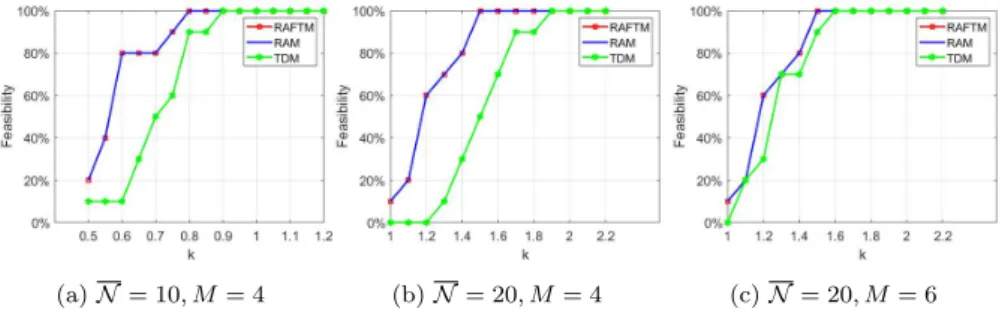
Fig. 1: Feasibility for a) N = 10, M = 4, b) N = 20, M = 4, and c) N = 20, M = 6 for all DVFS schemes.
To evaluate the approaches, the following metrics are used:
1. Feasibility, i.e., percentage of experiments that found the optimal solution in these 10 experiments.
2. Energy consumption of RAM and TDM, compared to the energy consump- tion of the proposed RAFTM approach.
3. Reliability Improvement (RI =Ri−Rthi ), i.e., the task reliabilityabovethe reliability threshold.
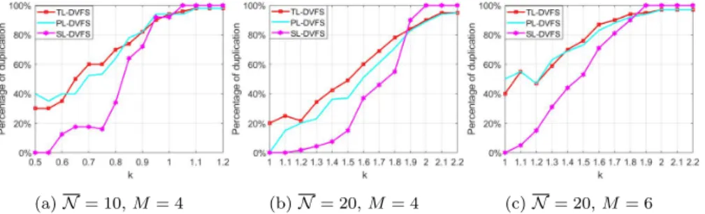
4. Task duplication, i.e., the percentage of tasks that RAFTM decided to duplicate.
5. Time, i.e., the time required for each approach to find a solution.
To better explain the performance, we organize our experiments in two set-ups of reliability threshold:
1. Set-up 1: The task reliability threshold can always be met by executing only the original task using a high processor frequency. To achieve that, the reliability threshold is selected within [0.9990,0.9995] and the average failure rateλ0 equal to 5×10⁻⁵faults/sec. In this set-up, the feasibility of RAFTM and RAM are the same.
2. Set-up 2: The task reliability threshold cannot always be met by execut- ing only the original task, even at maximum frequency. To achieve that, the range of reliability constraint is increased, i.e., [0.9990,0.9999]. We ex- plore the behavior of the proposed RAFTM and RAM approaches with the average failure rateλ0is equal to 5×10⁻⁵, 4×10⁻⁴, and 5×10⁻⁴faults/sec.
4.2 Experimental set-up 1
(a)N = 10,M= 4 (b)N = 20,M= 4 (c)N= 20,M= 6
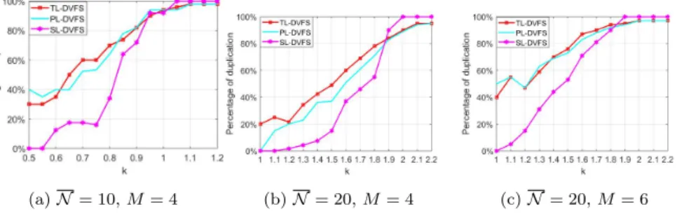
Fig. 2: RAFTM duplication percentage: a) N = 10, M = 4, b) N = 20, M = 4, and c)N = 20,M = 6 (all DVFS schemes).
4.2.1 Feasibility
The feasibility of RAFTM, RAM and TDM is depicted in Fig. 1, forN = 10 andN = 20 withM = 4, and forN = 20 withM = 6.
Regarding the comparison with TDM, RAFTM is able to find solutions in significantly more experiments than TDM, since RAFTM is not obliged to duplicate reliable tasks, compared to TDM. When feasibility is not 100% for both approaches, RAFTM can find a solution, on average, in 30%, 33% and 10% more experiments, than TDM (Fig. 1). When k = 1,1.1,1.2 (N = 20 and M = 4), TDM cannot find any solution. As the number of processors is increased, e.g., fromM = 4 toM = 6, the capability of TDM to find solutions improves, as more cores are available to schedule the duplicated tasks. Note that RAFTM achieves 100% feasibility in earlier deadlines than TDM, i.e., k = 0.8 (N = 10 andM = 4) and k = 1.5 (N = 20 and M = 4, N = 20 andM = 6). When the deadline becomes relaxed (and TDM canalways find solutions), i.e.,k= 0.9 (N = 10 andM = 4),k= 1.9 (N = 20 andM = 4),
(a) TL-DVFS (N = 10,M= 4)
(b) PL-DVFS (N = 10,M = 4)
(c) SL-DVFS (N = 10,M = 4)
(d) TL-DVFS (N = 20,M= 4)
(e) PL-DVFS (N = 20,M = 4)
(f) SL-DVFS (N = 20,M = 4)
(g) TL-DVFS (N = 20,M= 6)
(h) PL-DVFS (N = 20,M = 6)
(i) SL-DVFS (N = 20, M = 6)
Fig. 3: Energy Consumption (EC) gain: N = 10, M = 4 (a, b, c), N = 20, M = 4 (d, e, f), andN = 20,M = 6 (g, h, i).
and k = 1.6 (N = 20 andM = 6), RAFTM has a similar behaviour with TDM, since it decides to duplicate the majority of the tasks, achieving similar gains, as explained in the next section.
Regarding the comparison with RAM, in this experimental set-up, RAFTM and RAM have the same feasibility, since the reliability constraints can always be met by executing only the original task with a high processor frequency.
Note that, we explore the difference of feasibility between RAFTM and RAM, in the experimental set-up 2, where high frequencies cannot always satisfy reliability thresholds. We observe that the feasibility of RAFTM and RAM is not modified as the number of cores is increased, due to the dependencies of the task graph. However, since TDM requires to duplicate all tasks, its feasibility is increased with more processors, approaching the RAFMT and RAM feasibility with 6 processors.
(a) TL-DVFS (N = 10,M= 4)
(b) PL-DVFS (N = 10,M = 4)
(c) SL-DVFS (N = 10,M = 4)
(d) TL-DVFS (N = 20,M= 4)
(e) PL-DVFS (N = 20,M = 4)
(f) SL-DVFS (N = 20,M = 4)
(g) TL-DVFS (N = 20,M= 6)
(h) PL-DVFS (N = 20,M = 6)
(i) SL-DVFS (N = 20, M = 6)
Fig. 4: Reliability improvement: N = 10, M = 4 (a,b,c), N = 20, M = 4 (d,e,f), andN = 20,M = 6 (g,h,i).
4.2.2 Energy consumption
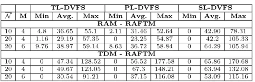
The energy consumption of RAM and TDM, compared to the proposed ap- proach, is depicted in Fig. 3. The minimum, average and maximum gains
Table 4: Min, avg. and max energy gains (%)
TL-DVFS PL-DVFS SL-DVFS
N M Min Avg. Max Min Avg. Max Min Avg. Max RAM - RAFTM
10 4 4.8 36.65 55.1 2.11 31.46 52.64 0 42.90 78.31 20 4 1.16 29.19 57.35 0 23.25 54.87 0 42.2 105.33 20 6 9.76 38.97 59.14 8.63 36.72 58.84 0 64.29 105.94
TDM - RAFTM
10 4 0 47.34 128.52 0 56.52 177.58 0 65.86 170.68 20 4 0 49.67 123.05 0 67.3 148.21 0 63.94 132.08 20 6 0 30.54 91.21 0 37.15 116.08 0 53.09 115.16
are depicted in Table 4. Note that, the minimum gain is 0 between TDM and RAFTM, when the deadlines are less strict. When deadline is relaxed, RAFTM performs duplication for all tasks, as TDM. For RAM, we observe a minimum gain of 0, only in very few strict deadlines, either with a high number of tasks or due to SL-DVFS, where the frequency assignment is very restricted. In the strict deadlines, RAFTM and RAM have a similar behavior: applying a high frequency to meet the timing constraint, thus no duplication is possible. From the obtained results, we can make the following general observations:
– When the number of tasks is increased from N = 10 toN = 20 with the same number of cores (from Fig. 3a to Fig. 3d, from Fig. 3b to Fig. 3e, and from Fig. 3c to Fig. 3f), the energy savings remain high for the pro- posed RAFTM approach, compared to RAM and TDM. We observe a slight decrease in average savings regarding RAM in TL-DVFS and PL-DVFS schemes, due to the fact that RAFTM behaves as RAM in very strict dead- lines. On the one hand, RAM consumes more energy compared to RAFTM, as Table 4 shows. On the other hand, RAFTM is able to find solutions in more cases, compared to TDM, especially for strict deadlines, as Fig. 1 shows.
– When the number of cores increases from M = 4 toM = 6, with the same number of tasksN = 20, (from Fig. 3d to Fig. 3g, from Fig. 3e to Fig. 3h, and from Fig. 3f to Fig. 3i), the energy savings of RAFTM compared to RAM are enlarged, on average, to 38.9% (TL-DVFS), 36.72% (PL-DVFS), and 64.29% (SL-DVFS). This is supported by the fact that when more resources like processors are available, our proposed approach has more freedom to use the available processors when performing the task mapping, minimizing the total energy consumption.
– Among different DVFS schemes, we observed that SL-DVFS has a higher impact on the observed gains of RAFTM vs RAM, compared to the im- pact it has on the observed gains of RAFTM vs TDM, as the number of tasks and cores increases. When the supported DVFS scheme is flexible, RAM performs a more fine-grained assignment, achieving a lower energy consumption. However, when SL-DVFS is supported, RAM is obliged to select a high frequency in order to meet the highest reliability threshold of the tasks and executes all tasks with this high frequency, causing large energy consumption. On the other hand, the proposed RAFTM can exploit task duplication, applying a lower frequency, and thus, reducing the energy consumption, when time slack is available for relaxed deadline cases.
With a more detailed observation, when both RAFTM and TDM ap- proaches can find solutions, RAFTM provides a solution that consumes sig- nificantly less energy. More precisely, whenN = 20 andM = 4, for TL-DVFS we observe a maximum gain of 123.05%, with an average gain of 49.67%, for PL-DVFS, we observe a maximum gain of 148.21% with an average gain of 67.3%, and, for SL-DVFS, there is a maximum gain 132.08%, with an average gain of 63.94%.
Furthermore, RAFTM finds a solution, that consumes less energy than RAM, since RAFTM can duplicate some tasks in order to use lower frequen- cies, reducing energy consumption. When the deadline is not so strict (part of graph with almost flat average gain in the box-plot of Fig. 3), the highest energy gains are observed. More precisely, whenM = 4, we observe an average gain of 54.01% (TL-DVFS), 50.5% (PL-DVFS), and 73.48% (SL-DVFS) for N = 10 and an average gain of 54.27% (TL-DVFS), 48.88% (PL-DVFS), and 92.19% (SL-DVFS) for N = 20. When M = 6 and N = 20, the observed average gain is 57.98% (TL-DVFS), 57.06% (PL-DVFS), and 102.11% (SL- DVFS). For very strict deadlines, the energy gains of RAFTM and RAM are similar; RAFTM behaves as RAM, since there is no available time slack, and thus, RAFTM assigns high frequencies, without task duplication. We observe minimum gains when k = 0.5 (N = 10) and k = 1 (N = 20). When SL- DVFS and less cores are used (M = 4), RAFTM cannot exploit duplication and use different frequencies to reduce energy consumption, and thus, it be- haves as RAM. When time slack exists, RAFTM can take advantage of it and duplicate some tasks, if energy gains can be achieved.
(a)N = 10,M= 4 (b)N = 20,M= 4 (c)N= 20,M= 6
Fig. 5: RAFTM duplication percentage: a) N = 10, M = 4, b) N = 20, M = 4, and c)N = 20,M = 6 (all DVFS schemes).
4.2.3 Reliability Improvement
We also compare the reliability improvement with regard to the reliability threshold in Fig. 4, for the three DVFS schemes and forN = 10 andN = 20, withM=4, andN = 20, withM=6. Generally:
– Regarding RAM, when TL-DVFS is considered, it has the lowest reliability improvement. This is because RAM only requires to meet the reliability threshold in order to find a solution. However, when PL-DVFS and SL- DVFS are considered, RAM is obliged to select a higher frequency, even for tasks with lower reliability threshold, due to the restrictions in the DVFS schemes. As a result, the reliability improvement of RAM is increased, when the DVFS schemes are more restricted. Note that, when the number of tasks
is increased in SL-DVFS, RAM is obliged to always select high frequencies to meet the highest reliability threshold, among all tasks, and then, use this frequency for task execution, even if time slack exists.
– Regarding RAFTM, it provides higher reliability improvements than RAM, for all deadlines. For tight deadlines, it provides lower reliability improve- ments than TDM, as it partially duplicates the task set. However, as dis- cussed in the previous section, RAFTM is more capable of finding solu- tions compared to TDM, and with significantly reduced energy consump- tion. When the deadline is not so strict, it provides the same reliability improvements as TDM, since they behave in a similar way.
– Regarding TDM, since it always duplicates the tasks, it provides a high reliability improvement, if it can find a solution. Therefore, going from TL- DVFS to PL-DVFS and SL-DVFS, does not have a high impact on the reliability improvement. Moreover, when a solution is found in strict dead- lines, it has typically significant reliability improvement, at the price of high energy consumption, since high frequencies are required to meet the strict timing constraints.
Table 5: Running time (seconds), when at least one solution is found, with N = 10,M = 4
deadline(k) 0.5 0.55 0.6 0.65 0.7 0.75 0.8 0.85 0.9 0.95 1 1.05 1.1 1.15 1.2 TL DVFS
RAFTM 0.45 0.57 0.95 2.17 3.31 4.31 3.77 3.11 5.57 1.47 1.92 3.71 0.51 0.3 0.27 RAM 0.3 0.25 0.27 0.22 0.43 0.33 0.16 0.16 0.21 0.18 0.18 0.16 0.19 0.16 0.19 TDM 2.52 0.56 0.61 0.97 1.53 2.65 2.45 2.08 1.26 1.08 0.72 0.72 0.55 0.36 0.37 PL DVFS
RAFTM 1.65 6.03 8.2 15.26 24.06 32.3 34.38 40.76 29.12 29.05 13.9 13.54 10.94 4.19 3.51 RAM 0.82 1.78 1.51 1.7 1.94 1.72 1.79 1.79 2.15 2.22 1.87 1.88 2.1 1.77 1.84 TDM 2.55 2.27 1.7 4.45 5.97 9.17 5.04 4.97 4.83 3.61 3.22 2.47 2.34 1.84 1.87 SL DVFS
RAFTM 0.28 0.19 0.26 0.83 1.47 1.86 1.18 1.13 0.84 0.92 0.67 0.59 0.53 0.27 0.23 RAM 0.11 0.08 0.11 0.09 0.19 0.2 0.2 0.07 0.09 0.08 0.08 0.09 0.09 0.08 0.08 TDM 0.48 0.14 1.02 1.64 1.51 2.5 1.83 1.59 1.43 1.7 0.88 0.68 0.71 0.54 0.44
Table 6: Running time (seconds), when at least one solution is found, with N = 20,M = 4
deadline(k) 1.0 1.1 1.2 1.3 1.4 1.5 1.6 1.7 1.8 1.9 2.0 2.1 2.2 TL DVFS
RAFTM 14.9 61 74.9 138.2 202.1 256.9 327.3 219 1039.3 1054.7 126.8 58.7 123.1 RAM 0.07 0.04 0.067 0.054 0.041 0.061 0.066 0.045 0.043 0.036 0.053 0.052 0.044 TDM - - - 9188.3 1550.4 1015.9 1165.4 2304.7 2814.6 1350.6 700.6 549.3 237.8 PL DVFS
RAFTM 228.6 662.2 529.9 1092 1815 4665 15722 4676 33294 70465 24239 24054 24072 RAM 84.3 99.2 44.4 74.3 76.5 65.5 52.4 55 56.3 41.7 42.8 57.4 56.3 TDM - - - 2740 5677.5 5084.1 9641.1 14770.4 10571.4 8235.2 5517.1 3619.0 3169.6 SL DVFS
RAFTM 0.53 0.3 5.76 14.14 21.69 98.22 91.88 183.39 1301.28 585.03 65.29 28.56 15.08 RAM 0.08 0.06 0.038 0.069 0.045 0.066 0.059 0.036 0.027 0.026 0.025 0.037 0.025 TDM - - - 238.51 230.59 230.59 230.59 230.59 230.59 230.59 230.59 230.59 230.59
Table 7: Running time (seconds), when at least one solution is found, with N = 20,M = 6
deadline(k) 1.0 1.1 1.2 1.3 1.4 1.5 1.6 1.7 1.8 1.9 2.0 2.1 2.2 TL DVFS
RAFTM 0.8 58.1 26.9 89.9 81.9 109.8 58.6 62.8 59.8 14.7 2.5 0.7 0.6 RAM 0.07 0.06 0.08 0.09 0.10 0.06 0.05 0.05 0.07 0.05 0.06 0.08 0.05 TDM - 70.8 333.4 124.4 298.2 227.4 70.5 160.6 203.4 39.8 2.9 1.4 0.9 PL DVFS
RAFTM 114.2 697.3 730.8 661.5 859.5 824.0 1090.1 503.3 569.2 188.6 95.9 82.5 75.0 RAM 566.0 397.9 533.6 671.5 546.1 820.5 954.5 562.0 687.4 693.2 799.0 1113.8 700.0 TDM - 2861.2 2874.1 5312.8 8795.7 1477.3 1237.6 1243.7 1794.6 232.5 41.7 42.2 35.2 SL DVFS
RAFTM 0.4 0.3 1.4 12.1 12.6 23.5 19.2 19.7 16.1 21.3 5.9 4.7 5.6 RAM 0.09 0.07 0.06 0.12 0.08 0.06 0.04 0.04 0.04 0.04 0.04 0.05 0.04 TDM - 8.7 111.0 37.8 71.9 83.0 52.3 52.6 41.9 32.8 19.5 20.2 16.3
4.2.4 RAFTM duplication
Fig. 5 depicts the task duplication obtained by the proposed approach. RAM approach does not apply duplication for any task (0%) and TDM duplicates all tasks (100%). Generally observed for all DVFS schemes, when the dead- line is more relaxed, RAFTM can duplicate more tasks using lower frequency, thus achieving less energy consumption, due to the available time slack. Fur- thermore, as all processors have the same frequency in SL-DVFS, this DVFS scheme has less flexibility in task duplication and scheduling, when deadlines are strict. In Fig. 5, there are two interesting observations: i) for some points, the duplication percentage decreases, when deadline is relaxed (Fig. 5b, when k = 1.2 for TL-DVFS, and Fig. 5c, when k = 1.2 for both TL/PL-DVFS), and ii) the duplication percentage does not reach 100% for TL/PL-DVFS, as SL-DVFS does. The reason is the flexibility to decide the task frequency for different DVFS schemes, and the reliability threshold’s value. When the task’s reliability threshold can be satisfied without duplication and with a low fre- quency, and energy consumption is less than the energy consumption when duplicating with the lowest frequency, then TL-DVFS and PL-DVFS schemes do not duplicate the task. However, with SL-DVFS, the same frequency must be assigned to all processors. Hence, a task with a high reliability constraint forces other tasks with low reliability constraints to execute with a higher frequency than the required one. As a result, duplication does not provide benefits, even if time slack exists. Due to these reasons, the duplication per- centage is usually smaller for SL-DVFS, compared to TL/PL-DVFS, except for relaxed enough deadlines.
4.2.5 Time
Tables 5 to 7 provide the time required to find a solution, when N = 10 and N = 20 with M = 4, and N = 20 with M = 6. Comparing Table 6
and Table 5, with more tasks, more time is required to find a solution, as expected. For RAFTM, when deadline is very strict or very relaxed, less time is needed to obtain the solutions. However, with intermediate deadlines, more time is required as RAFTM needs to explore the available time slack to decide which, and how many, tasks to be duplicated, without violating constraints, while consuming the least energy. TDM is the most running time expensive approach, because all tasks need to be duplicated, increasing the number of tasks to be scheduled, and thus, the time to find the solutions. Although RAM is the least running time expensive approach, it provides less energy savings.
4.3 Experimental set-up 2
In this experimental set-up, we explore the behavior of RAFTM and RAM at different failure ratesλ0under TL-DVFS scheme. First, we extend the range of the task reliability threshold, in order to have few tasks with higher reliability requirements. Then, we tune the parameter λ0 in order to change the failure rate. This experimental set-up shows how the fault model influences the ability of obtaining feasible solutions, through a slight increase ofλ0. The results show that the proposed approach provides better results than RAM, with the fault rate changing. These modifications will affect only the proposed RAFTM and RAM approaches, since they use the reliability constraint to decide the task mapping. The results of TDM remain similar to the previous section.
4.3.1 Feasibility
The first column of Fig. 6 depicts the ability of RAM, compared to RAFTM, to obtain feasible solution, forλ0= 4×10⁻⁴(Fig. 6a and Fig. 6c) andλ0= 5×10⁻⁴ (Fig. 6b and Fig. 6d), withN = 10 andN = 20,M = 4. Generally:
– As theλ0increases, the reliability of a task, due to the processor fault rate, is decreased. Therefore, withλ0increasing, the capability of RAM to always find a frequency, that meets the reliability threshold of all tasks, decreases, especially for tasks with high reliability requirements. Furthermore, even with λ0 increasing, RAFTM is able to still meet these high reliability re- quirements, by duplicating tasks and assigning a high frequency. This can be observed by comparing Fig. 6a to Fig. 6d, where the feasibility of RAM is reduced by 20%, and Fig. 6g to Fig. 6j, where the feasibility of RAM is reduced by 30%. However, RAFTM feasibility remains the same, always finding a solution at relaxed deadlines.
– As the number of tasks increases, the feasibility is affected. As we observe by comparing Fig. 6a to Fig. 6g and Fig. 6d to Fig. 6j, the curves of RAM and RAFTM separate at stricter deadlines, whenN = 20, compared to the ones whenN = 10. Comparing the feasibility between set-up 1 and set-up 2, we observe that the feasibility of set-up1 can be 100% for both RAFTM and RAM, with a smaller average fault rateλ0 at relaxed deadlines. How- ever, with the average fault rate increasing, it is not possible for RAM to
(a)λ0= 4×10⁻⁴(N = 10) (b)λ0= 4×10⁻⁴(N= 10) (c)λ0= 4×10⁻⁴(N = 10)
(d)λ0= 5×10⁻⁴(N = 10) (e)λ0= 5×10⁻⁴(N = 10) (f)λ0= 5×10⁻⁴(N = 10)
(g)λ0= 4×10⁻⁴(N = 20) (h)λ0= 4×10⁻⁴(N= 20) (i)λ0= 4×10⁻⁴(N = 20)
(j)λ0= 5×10⁻⁴(N= 20) (k)λ0= 5×10⁻⁴(N= 20) (l)λ0= 5×10⁻⁴(N = 20)
Fig. 6: TL-DVFS: Feasibility (first column), Energy Consumption (EC) gain (second column) and Reliability Improvement (RI) (third column) for λ0 = 4×10⁻⁴andλ0= 5×10⁻⁴, withN = 10 andN = 20 (M = 4).
find a solution satisfying the reliability requirements, even with maximum frequency and relaxed deadline. This observation worsens withλ0 increas- ing. Thus, with a different fault model, executing only the original task may not be able to provide reliable execution. Therefore, replication is needed in order to guarantee the reliability threshold of the tasks.
4.3.2 Energy consumption
The second column of Fig. 6 depicts the energy consumption of RAM, com- pared to the proposed approach, when RAM found a solution.
– As theλ0increases, the processor sensibility to faults is increased. Then, the energy gains are slightly reduced, from 12.05% to 8.87% (N = 10, Fig. 6b to Fig. 6e) and from 12.60% to 10.75% (N = 20), Fig. 6h to Fig. 6k, since RAFTM also selects a high frequency, in order to meet the high reliability thresholds of tasks.
– As the number of tasks increases, the gains in energy consumption remain similar. As we observe by comparing Fig. 6b to Fig. 6h and Fig. 6e to Fig. 6k, the energy savings are decreased, compared to set-up 1. For in- stance, from 36.65% (set-up 1) to 12.05% and 8.87%, when N = 10 and M = 4. This is due to the fact that, based onλ(f) (see Section 2.3), the reliability with same frequency decreases, when λ0 increases. In order to guarantee a reliable execution, a high frequency must be assigned to meet the reliability requirement, leading to higher energy consumption for the proposed approach.
4.3.3 Reliability improvement
The third column of Fig. 6 depicts the reliability improvement of RAFTM and RAM, for the cases where RAM was able to find a solution. On the basis of satisfying the reliability requirements, RAM achieves a slightly better reliability improvement than our approach, while it sacrifices the ability of obtaining feasible solutions.
Table 8: Running time (seconds), when at least one solution is found, with N = 10,M = 4 (TL-DVFS)
deadline(k) 0.5 0.55 0.6 0.65 0.7 0.75 0.8 0.85 0.9 0.95 1 1.05 1.1 1.15 1.2 λ0= 4×10⁻⁴ RAFTM 0.77 0.93 1.01 1.49 1.48 2.00 1.28 1.31 1.21 0.74 0.68 0.66 0.62 0.64 0.62
RAM 0.07 0.04 0.06 0.07 0.13 0.19 0.12 0.05 0.06 0.05 0.06 0.06 0.05 0.04 0.04 λ0= 5×10⁻⁴ RAFTM 0.67 0.61 0.87 1.18 0.87 1.39 0.80 0.72 0.66 0.55 0.53 0.58 0.55 0.57 0.50 RAM 0.10 0.05 0.05 0.06 0.13 0.20 0.13 0.05 0.05 0.08 0.05 0.05 0.05 0.04 0.07
Table 9: Running time (seconds), when at least one solution is found, with N = 20,M = 4 (TL-DVFS)
deadline(k) 1.0 1.1 1.2 1.3 1.4 1.5 1.6 1.7 1.8 1.9 2.0 2.1 2.2 λ0= 4×10⁻⁴ RAFTM 26.85 194.76 98.45 208.45 224.04 315.23 167.25 326.79 278.74 99.46 216.81 31.26 4.79
RAM 0.04 0.03 0.02 0.05 0.03 0.04 0.04 0.04 0.03 0.02 0.02 0.03 0.02 λ0= 5×10⁻⁴ RAFTM 32.08 206.57 583.86 156.99 155.10 117.55 155.63 174.00 19.15 24.26 33.65 3.52 3.06 RAM 0.05 0.03 0.03 0.05 0.04 0.05 0.05 0.04 0.04 0.02 0.03 0.04 0.02