HAL Id: hal-00941144
https://hal.archives-ouvertes.fr/hal-00941144
Preprint submitted on 3 Feb 2014
HAL
is a multi-disciplinary open access archive for the deposit and dissemination of sci- entific research documents, whether they are pub- lished or not. The documents may come from teaching and research institutions in France or
L’archive ouverte pluridisciplinaire
HAL, estdestinée au dépôt et à la diffusion de documents scientifiques de niveau recherche, publiés ou non, émanant des établissements d’enseignement et de recherche français ou étrangers, des laboratoires
Finding Optimal Strategies of Almost Acyclic Simple Stochatic Games
David Auger, Pierre Coucheney, Yann Strozecki
To cite this version:
David Auger, Pierre Coucheney, Yann Strozecki. Finding Optimal Strategies of Almost Acyclic Simple
Stochatic Games. 2014. �hal-00941144�
Finding Optimal Strategies of Almost Acyclic Simple Stochatic Games
David Auger, Pierre Coucheney, Yann Strozecki
{david.auger, pierre.coucheney, yann.strozecki}@uvsq.fr PRiSM, Universit´e de Versailles Saint-Quentin-en-Yvelines
Versailles, France Abstract
The optimal value computation for turned-based stochastic games with reachability objectives, also known as simple stochastic games, is one of the few problems inNP∩coNPwhich are not known to be inP. However, there are some cases where these games can be easily solved, as for instance when the underlying graph is acyclic. In this work, we try to extend this tractability to several classes of games that can be thought as ”almost”
acyclic. We give some fixed-parameter tractable or polynomial algorithms in terms of different parameters such as the number of cycles or the size of the minimal feedback vertex set.
keywords: algorithmic game theory · stochastic games · FPT algorithms
Introduction
Asimple stochastic game, SSG for short, is a zero-sum, two-player, turn-based version, of the more generalstochastic games introduced by Shapley [17]. SSGs were introduced by Condon [6] and they provide a simple framework that allows to study the algorithmic complexity issues underlying reachability objectives.
A SSG is played by moving a pebble on a graph. Some vertices are divided between players MIN and MAX: if the pebble attains a vertex controlled by a player then he has to move the pebble along an arc leading to another vertex.
Some other vertices are ruled by chance; typically they have two outgoing arcs and a fair coin is tossed to decide where the pebble will go. Finally, there is a special vertex named the 1-sink, such that if the pebble reaches it player MAX wins, otherwise player MIN wins.
Player MAX’s objective is, given a starting vertex for the pebble, to maxi- mize the probability of winning against any strategy of MIN. One can show that it is enough to consider stationary deterministic strategies for both players [6].
Though seemingly simple since the number of stationary deterministic strate- gies is finite, the task of finding the pair of optimal strategies, or equivalently, of computing the so-calledoptimal values of vertices, is not known to be in P.
SSGs are closely related to other games such as parity games or discounted payoff games to cite a few [2]. Interestingly, those games provide natural appli- cations in model checking of the modalµ-calculus [18] or in economics. While it is known that they can be reduced to simple stochastic games [4], hence seem- ingly easier to solve, so far no polynomial algorithm are known for these games either.
Nevertheless, there are some very simple restrictions for SSGs for which the problem of finding optimal strategies is tractable. Firstly, if there is only one player, the game is reduced to a Markov Decision Process (MDP) which can be solved by linear programming. In the same vein, if there is no randomness, the game can be solved in almost linear time [1].
As an extension of that fact, there is a Fixed Parameter Tractable (FPT) algorithm, where the parameter is the number of average vertices [11]. The idea is to get rid of the average vertices by sorting them according to a guessed order. Finally, when the (graph underlying the) game is a directed acyclic graph (DAG), the values can be found in linear time by computing them backwardly from sinks.
Without the previous restrictions, algorithms running in exponential time are known. Among them, the Hoffman-Karp [13] algorithm proceeds by suc- cessively playing a local best-response named switch for one player, and then a global best-response for the other player. Generalizations of this algorithm have been proposed and, though efficient in practice, they fail to run in polynomial time on a well designed example [9], even in the simple case of MDPs [8]. These variations mainly concern the choice of vertices to switch at each turn of the al- gorithm which is quite similar to the choice of pivoting in the simplex algorithm for linear programming. This is not so surprising since computing the values of an SSG can be seen as a generalization of solving a linear program. The best algorithm so far is a randomized sub-exponential algorithm [15] that is based on an adaptation of a pivoting rule used for the simplex.
Our contribution
In this article, we present several graph parameters such that, when the pa- rameter is fixed, there is a polynomial time algorithm to solve the SSG value problem. More precisely, the parameters we look at will quantify how close to a DAG is the underlying graph of the SSG, a case that is solvable in linear time.
The most natural parameters that quantify the distance to a DAG would be one of the directed versions of the tree-width such as the DAG-width. Unfortu- nately, we are not yet able to prove a result even for SSG of bounded pathwidth.
In fact, in the simpler case of parity games the best algorithms for DAG-width and clique-width are polynomials but not even FPT [16, 3]. Thus we focus on restrictions on the number of cycles and the size of a minimal feedback vertex set.
First, we introduce in Section 2 a new class of games, namelyMAX-acyclic games, which contains and generalizes the class of acyclic games. We show that the standard Hoffman-Karp algorithm, also known as strategy iteration algo- rithm, terminates in a linear number of steps for games in this class, yielding a polynomial algorithm to compute optimal values and strategies. It is known that, in the general case, this algorithm needs an exponential number of steps to compute optimal strategies, even in the simple case of Markov Decision Pro- cesses [8, 9].
Then, we extend in Section 3 this result to games with very few cycles, by giving an FPT-algorithm where the parameter is the number of fork vertices which bounds the number of cycles. To obtain a linear dependance in the total number of vertices, we have to reduce our problem to several instances of acyclic games since we cannot even rely on computing the values in a general game.
Finally, in Section 4, we provide an original method to “eliminate” vertices in an SSG. We apply it to obtain a polynomial time algorithm for the value problem on SSGs with a feedback vertex set of bounded size (Theorem 8).
1 Definitions and standard results
Simple stochastic games are turn-based stochastic games with reachability ob- jectives involving two players named MAX and MIN. In the original version of Condon [6], all vertices except sinks have outdegree exactly two, and there are only two sinks, one with value 0 and another with value 1. Here, we allow more than two sinks with general rational values, and more than an outdegree two for positional vertices.
Definition 1 (SSG). A simple stochastic game (SSG) is defined by a directed graph G = (V, A), together with a partition of the vertex set V in four parts VM AX, VM IN, VAV E and VSIN K. To every x ∈ VSIN K corresponds a value Val(x) which is a rational number in [0,1]. Moreover, vertices of VAV E have outdegree exactly 2, while sink vertices have outdegree 1 consisting of a single loop on themselves.
In the article, we denote by nM, nm and na the size of VM AX, VM IN and VAV E respectively and bynthe size ofV. The set ofpositional vertices, denoted VP OS, is VP OS =VM AX ∪VM IN. We now define strategies which we restrict to be stationary and pure, which turns out to be sufficient for optimality. Such strategies specify for each vertex of a player the choice of a neighbour.
Definition 2 (Strategy). A strategy for player MAX is a mapσ from VM AX
toV such that
∀x∈VM AX, (x, σ(x))∈A.
Strategies for player MIN are defined analogously and are usually denoted by τ. We denote Σ and T the sets of strategies for players MAX and MIN respectively.
Definition 3 (play). A play is a sequence of vertices x0, x1, x2, . . . such that for allt≥0,
(xt, xt+1)∈A.
Such a play is consistentwith strategiesσ and τ, respectively for player MAX and player MIN, if for all t≥0,
xt∈VM AX ⇒xt+1=σ(xt) and
xt∈VM IN ⇒xt+1=τ(xt).
A couple of strategiesσ, τ and an initial vertex x0 ∈V define recursively a random play consistent withσ, τ by setting:
• ifxt∈VM AX thenxt+1=σ(xt);
• ifxt∈VM IN thenxt+1 =τ(xt);
• ifxt∈VSIN K thenxt+1=xt;
• if xt ∈ VAV E, then xt+1 is one of the two neighbours of xt, the choice being made by a fair coin, independently of all other random choices.
Hence, two strategiesσ, τ, together with an initial vertexx0define a measure of probabilityPxσ,τ0 on plays consistent withσ, τ. Note that if a play contains a sink vertexx, then at every subsequent time the play stays in x. Such a play is said toreach sink x. To every playx0, x1, . . . we associate a value which is the value of the sink reached by the play if any, and 0 otherwise. This defines a random variable X once two strategies are fixed. We are interested in the expected value of this quantity, which we call the value of a vertexx∈V under strategiesσ, τ:
Valσ,τ(x) =Exσ,τ(X)
where Exσ,τ is the expected value under probability Pxσ,τ. The goal of player M AXis to maximize this (expected) value, and the best he can ensure against a strategyτ is
Valτ(x) = max
σ∈ΣValσ,τ(x)
while againstσplayer MIN can ensure that the expected value is at most Valσ(x) = min
τ∈TValσ,τ(x).
Finally, the value of a vertexx, is the common value Val(x) = max
σ∈Σmin
τ∈TValσ,τ(x) = min
τ∈Tmax
σ∈ΣValσ,τ(x). (1)
The fact that these two quantities are equal is nontrivial, and it can be found for instance in [6]. A pair of strategiesσ∗, τ∗ such that, for all verticesx,
Valσ∗,τ∗(x) = Val(x)
always exists and these strategies are said to beoptimal strategies. It is polynomial- time equivalent to compute optimal strategies or to compute the values of all vertices in the game, since values can be obtained from strategies by solving a linear system. Conversely if values are known, optimal strategies are given by greedy choices in linear time (see [6] and Lemma 1). Hence, we shall simply write ”solve the game” for these tasks.
We shall need the following notion:
Definition 4(Stopping SSG). A SSG is said to bestoppingif for every couple of strategies all plays eventually reach a sink vertex with probability1.
Condon [6] proved that every SSGGcan be reduced in polynomial time into a stopping SSGG′ whose size is quadratic in the size of G, and whose values almost remain the same.
Theorem 1(Optimality conditions, [6]). LetGbe a stopping SSG. The vector of values(Val(x))x∈V is the only vectorw satisfying:
• for everyx∈VM AX,w(x) = max{w(y)|(x, y)∈A};
• for everyx∈VM IN,w(x) = min{w(y)|(x, y)∈A};
• for everyx∈VAV E w(x) = 12w(x1) +12w(x2)wherex1 andx2 are the two neighbours ofx;
• for everyx∈VSIN K,w(x) =Val(x).
If the underlying graph of an SSG is acyclic, then the game is stopping and the previous local optimality conditions yield a very simple way to compute values. Indeed, we can use backward propagation of values since all leaves are sinks, and the values of sinks are known. We naturally call these gamesacyclic SSGs.
Once a pair of strategies has been fixed, the previous theorem enables us to see the values as solution of a system of linear equations. This yields the following lemma, which is an improvement on a similar result in [6], where the bound is 4n instead of 6na2 .
Lemma 1. Let G be an SSG with sinks having rational values of common denominatorq. Then under any pair of strategiesσ, τ, the value Valσ,τ(x)of any vertexxcan be computed in timeO(nωa), where ω is the exponent of the matrix multiplication, and na the number of average (binary) vertices. Moreover, the value can be written as a rational number ab, with
0≤a, b≤6na2 ×q.
Proof. We sketch the proof since it is standard. First, one can easily compute all verticesxsuch that
Valσ,τ(x) = 0.
LetZ be the set of these vertices. Then:
• all AVE vertices inZ have all their neighbours inZ;
• all MAX (resp. MIN) verticesxinZ are such thatσ(x) (resp. τ(x)) is in Z.
To computeZ, we can start with the setZ of all vertices except sinks with positive value and iterate the following
• ifZ contains an AVE vertexxwith a neighbour out ofZ, removexfrom Z;
• ifZ contains a MAX (resp. MIN) vertex xwith σ(x) (resp. τ(x)) out of Z, removexfromZ.
This process will stabilize in at most n steps and compute the required set Z. Once this is done, we can replace all vertices of Z by a sink with value zero, obtaining a gameG′ where under σ, τ, the values of all vertices will be unchanged.
Consider now in G’ two corresponding strategies σ, τ (keeping the same names to simplify) and a positional vertexx. Letx′ be the first non positional vertex that can be reached from x under strategies σ, τ. Clearly, x′ is well defined and
Valσ,τ(x) = Valσ,τ(x′).
This shows that the possible values under σ, τ of all vertices are the values of average and sink vertices. The same is true if one average vertex has its two arcs towards the same vertex, thus we can forget those also. The value of an average vertex being equal to the average value of its two neighbours, we see that we can write a system
z=Az+b (2)
where
• z is thena-dimensional vector containing the values of average vertices
• Ais a matrix where all lines have at most two 12 coefficients, the rest being zeros
• b is a vector whose entries are of the form 0, p2qi or pi2q+pj, corresponding to transitions from average vertices to sink vertices.
Since no vertices but sinks have value zero, it can be shown that this system has a unique solution, i.e. matrix I−A is nonsingular, where I is the na- dimensional identity matrix. We refer to [6] for details, the idea being that
since inn−1 steps there is a small probability of transition from any vertex of G′ to a sink vertex, the sum of all coefficients on a line ofAn−1 is strictly less than one, hence the convergence of
X
k≥0
Ak = (I−A)−1.
Rewriting (2) as
2(I−A)z= 2b,
we can use Cramer’s rule to obtain that the valuezv of an average vertexv is zv= detBv
det 2(I−A)
whereBv is the matrix 2(I−A) with the column corresponding to v replaced by 2b. Hence by expanding the determinant we see that zv is of the form
1 det 2(I−A)
X
w∈VAV E
±2bwdet(2(I−A)v,w)
where 2(I−A)v,w is the matrix 2(I−A) where the line corresponding tovand the column corresponding towhave been removed.
Since 2bwhas either value 0, pqi or pi+pq j for some 1≤i, j≤na, we can write the value ofzv as a fraction of integers
P
w∈v±2bwq·det(2(I−A)v,w) det 2(I−A)·q
It remains to be seen, by Hadamard’s inequality, that since the nonzero entries of 2(I−A) on a line are a 2 and at most two−1, we have
det 2(I−A)≤6na2 , which concludes the proof.
The bound 6na2 is almost optimal. Indeed a caterpillar tree of n average vertices connected to the 0 sink except the last one, which is connected to the 1 sink, has a value of 12n at the root. Note that the lemma is slightly more general (rational values on sinks) and the bound a bit better (√
6 instead of 4) than what is usually found in the literature.
In all this paper, the complexity of the algorithms will be given in term of number of arithmetic operations and comparisons on the values as it is custom- ary. The numbers occurring in the algorithms are rationals of value at most exponential in the number of vertices in the game, therefore the bit complexity is increased by at most an almost linear factor.
2 MAX-acyclic SSGs
In this section we define a class of SSG that generalize acyclic SSGs and still have a polynomial-time algorithm solving the value problem.
A cycle of an SSG is anoriented cycle of the underlying graph.
Definition 5. We say that an SSG is MAX-acyclic(respectively MIN-acyclic) if from any MAX vertex x(resp. MIN vertex), for all outgoing arcs abut one, all plays going throughanever reach xagain.
Therefore this class contains the class of acyclic SSGs and we can see this hypothesis as being a mild form of acyclicity. From now on, we will stick to MAX-acyclic SSGs, but any result would be true for MIN-acyclic SSGs also.
There is a simple characterization of MAX-acyclicity in term of the structure of the underlying graph.
Lemma 2. An SSG is MAX-acyclic if and only if every MAX vertex has at most one outgoing arc in a cycle.
Let us specify the following notion.
Definition 6. We say that an SSG is strongly connected if the underlying directed graph, once sinks are removed, is strongly connected.
Lemma 3. Let G be a MAX-acyclic, strongly connected SSG. Then for each MAXx, all neighbours of xbut one must be sinks.
Proof. Indeed, if x has two neighbours y and z which are not sinks, then by strong connexity there are directed paths fromy toxand fromzto x. Hence, both arcs xy and xz are on a cycle, contradicting the assumption of MAX- acyclicity.
From now on, we will focus on computing the values of a strongly connected MAX-acyclic SSG. Indeed, it easy to reduce the general case of a MAX-acyclic SSG to strongly connected by computing the DAG of the strongly connected components in linear time. We then only need to compute the values in each of the components, beginning by the leaves.
We will show that the Hoffman-Karp algorithm [13, 7], when applied to a strongly connected MAX-acyclic SSG, runs for at most a linear number of steps before reaching an optimal solution. Let us remind the notion ofswitchability in simple stochastic games. Ifσis a strategy for MAX, then a MAX vertexxis switchable forσif there is an neighboury ofxsuch that Valσ(y)>Valσ(σ(x)).
Switching such a vertexxconsists in considering the strategyσ′, equal toσbut forσ′(x) =y.
For two vectorsv andw, we notev≥wif the inequality holds component- wise, andv > w if moreover at least one component is strictly larger.
Lemma 4 (See Lemma 3.5 in [19]). Let σ be a strategy for MAX and S be a set of switchable vertices. Letσ′ be the strategy obtained when all vertices of S are switched. Then
Valσ′ >Valσ.
Let us recall the Hoffman-Karp algorithm:
1. Letσ0 be any strategy for MAX andτ0 be a best response toσ0
2. while (σt, τt) is not optimal:
(a) let σt+1 be obtained from σt by switching one (or more) switchable vertex
(b) letτt+1 be a best response toσt+1
The Hoffman-Karp algorithm computes a finite sequence (σt)0≤t≤T of strate- gies for the MAX player such that
∀0≤t≤T−1, Valσt+1>Valσt.
If any MAX vertex x in a strongly connected MAX-acyclic SSG has more than one sink neighbour, says1, s2,· · ·sk, then these can be replaced by a single sink neighbours′ whose value is
Val(s′) := max
i=1..kVal(si).
Hence, we can suppose that all MAX vertices in a strongly connected MAX- acyclic SSG have degree two. For such a reduced game, we shall say that a MAX vertex xis open for a strategy σ ifσ(x) is the sink neighbour of xand thatxisclosed otherwise.
Lemma 5. Let G be a strongly connected, MAX-acyclic SSG, where all MAX vertices have degree 2. Then the Hoffman-Karp algorithm, starting from any strategyσ0, halts in at most 2nM steps. Moreover, starting from the strategy where every MAX vertex is open, the algorithm halts in at mostnM steps. All in all, the computation is polynomial in the size of the game.
Proof. We just observe that if a MAX vertex x is closed at time t , then it remains so until the end of the computation. More precisely, ifs:=σt−1(x) is a sink vertex, and y :=σt(x) is not, then since x has been switched we must have
Valσt(y)>Valσt(s).
For all subsequent timest′> t, since strategies are improving we will have Valσt′(y)≥Valσt(y)>Valσt(s) = Valσt′(s) = Val(s),
so thatxwill never be switchable again.
Thus starting from any strategy, if a MAX vertex is closed it cannot be opened and closed again, and if it is open it can only be closed once.
Each step of the Hoffman-Karp algorithm requires to compute a best-response for the MIN player. A best-response to any strategy can be simply computed with a linear program with as many variables as vertices in the SSG, hence in polynomial time. We will denote this complexity by O(nη); it is well known that we can haveη≤4, for instance with Karmarkar’s algorithm.
Theorem 2. A strongly connected MAX-acyclic SSG can be solved in time O(nMnη).
Before ending this part, let us note that in the case where the game is also MIN-acyclic, one can compute directly a best response to a MAX strategyσ without linear programming: starting with a MIN strategy τ0 where all MIN vertices are open, close all MIN verticesxsuch that their neighbour has a value strictly less than their sink. One obtains a strategyτ1such that
Valσ,τ1 <Valσ,τ0,
and the same process can be repeated. By a similar argument than in the previous proof, a closed MIN vertex will never be opened again, hence the number of steps is at most the number of MIN vertices, and each step only necessitates to compute the values, i.e. to solve a linear system (see Lemma 1).
Corollary 1. A strongly connected MAX and MIN-acyclic SSG can be solved in timeO(nMnmnω), whereω is the exponent of matrix multiplication.
3 SSG with few fork vertices
Work on this section has begun with Yannis Juglaret during his Master intern- ship at PRiSM laboratory. Preliminary results about SSGs with one simple cycle can be found in his report [14]. We shall here obtain fixed-parameter tractable (FPT) algorithms in terms of parameters quantifying how far a graph is from being MAX-acyclic and MIN-acyclic, in the sense of section 2. These parameters are:
kp= X
x∈VP OS
(|{y: (x, y)∈Aand is in a cycle}| −1) and
ka = X
x∈VAV E
(|{y: (x, y)∈Aand is in a cycle}| −1).
We say that an SSG is POS-acyclic (for positional acyclic) when it is both MAX and MIN-acyclic. Clearly, parameterkp counts the number of edges vio- lating this condition in the game. Similarly, we say that the game is AVE-acyclic when average vertices have at most one outgoing arc in a cycle. We call fork vertices, those vertices that have at least two outgoing arcs in a cycle. Since averages vertices have only two neighbours, ka is the number of fork average vertices.
Note that:
1. Whenkp= 0 (respectivelyka= 0), the game is POS-acyclic (resp. AVE- acyclic).
2. Whenka =kp = 0, the strongly connected components of the game are cycles. We study these games, which we call almost acyclic, in detail in subsection 3.1.
3. Finally, the number of simple cycles of the SSG is always less thankp+ka, therefore getting an FTP algorithm inkpandkaimmediately gives an FTP algorithm in the number of cycles.
We obtain:
Theorem 3. There is an algorithm which solves the value problem for SSGs in timeO(nf(kp, ka)), withf(kp, ka) =ka!4ka2kp.
As a corollary, by remark 3 above we have:
Theorem 4. There is an algorithm which solves the value problem for SSGs withk simple cycles in timeO(ng(k))with g(k) = (k−1)!4k−1.
Note that in both cases, when parameters are fixed, the dependance innis linear.
Before going further, let us explain how one could easily build on the previous part and obtain an FPT algorithm in parameter kp, but with a much worse dependance inn.
When kp > 0, one can fix partially a strategy on positional fork vertices, hence obtaining a POS-acyclic subgame that can be solved in polynomial time according to Corollary 1, using the Hoffman-Karp algorithm. Combining this with a bruteforce approach looking exhaustively through all possible local choices at positional fork vertices, we readily obtain a polynomial algorithm for the value problem whenkp is fixed:
Theorem 5. There is an algorithm to solve the value problem of an SSG in timeO(nMnmnω2kp).
We shall conserve this brute-force approach. In the following, we give an algorithm that reduces the polynomial complexity to a linear complexity when ka is fixed. From now on, up to applying the same bruteforce procedure, we assume kp = 0 (all fork vertices are average vertices). We also consider the case of a strongly connected SSG, since otherwise the problem can be solved for each strongly connected component as done in Section 2. We begin with the baselineka = 0 and extend the algorithm to general values ofka. Before this, we provide some preliminary lemmas and definitions that will be used in the rest of the section.
Apartial strategy is a strategy defined on a subset of vertices controlled by the player. Letσbe such a partial strategy for player MAX, we denote byG[σ]
the subgame of Gwhere the set of strategies of MAX is reduced to the ones that coincide withσon its support. According to equation (1), the value of an SSG is the highest expected value that MAX can guarantee, then it decreases with the set of actions of MAX:
Lemma 6. Let Gbe an SSG with value v, σ a partial strategy of MAX, and G[σ]the subgame induced byσ with valuev′. Thenv≥v′.
In strongly connected POS-acyclic games, positional vertices have at least one outgoing arc to a sink. Recall that, in case the strategy chooses a sink, we say that it is open at this vertex (the strategy is said open if it is open at a vertex), and closed otherwise. We can then compare the value of an SSG with that of the subgame generated by any open strategy.
Lemma 7. Let xbe a MAX vertex of an SSG Gwith a sink neighbour, andσ the partial strategy open atx. If it is optimal to openxinG, then it is optimal to open it inG[σ].
Proof. Since it is optimal to open xin G, the value of its neighbour sink is at least that of any neighbour vertex, sayy. But, in view of Lemma 6, the value ofyinG[σ] is smaller than inG, and then it is again optimal to play a strategy open atxin the subgame.
This lemma allows to reduce an almost acyclic SSG (resp. an SSG with parameterka >0) to an acyclic SSG (resp. an SSG with parameter ka−1).
Indeed, if the optimal MAX strategy is open at vertex x, then the optimal strategy of the subgame open at any MAX vertex will be open atx. A solution to find x once the subgame is solved (and then to reduce the parameterka) consists in testing all the open MAX vertices. But it may be the case that all MAX vertices are open which would not yield a FPT algorithm. In Lemma 8 (resp. Lemma 9), we give a restriction on the set of MAX vertices that has to be tested whenka= 0 (resp. ka >0) which provides an FPT algorithm.
3.1 Almost acyclic SSGs
We consider an SSG withka = 0. Together with the hypothesis that it is POS- acyclic and strongly connected, its graph, once sinks are removed, consists of a single cycle. A naive algorithm to compute the value of such SSG consists in looking for, if it exists, a vertex that is open in the optimal strategy, and then solve the acyclic subgame:
1. For each positional vertexx:
(a) compute the values of the acyclic SSG G[σ], where σ is the partial strategy open atx,
(b) if the local optimality condition is satisfied for x in G, return the values.
2. If optimal strategies have not been found, return the value when all vertices are closed.
This naive algorithm uses the routine that computes the value of an SSG with only one cycle. When the strategies are closed, the values can be computed in linear time as for an acyclic game. Indeed, letxbe an average vertex (if none, the game can be solved in linear time) ands1. . . sℓbe the values of the average neighbour sinks in the order given by a walk on the cycle starting fromx. Then
the value of x satisfies the equation Val(x) = 12s1+12(12s2+12(· · ·+ 12(12sℓ+
1
2Val(x)))), so that
Val(x) = 2ℓ 2ℓ−1
ℓ
X
i=1
2−isi, (3)
which can be computed in time linear in the size of the cycle. The value of the other vertices can be computed by walking backward from x, again in linear time. Finally, since solving an acyclic SSG is linear, the complexity of the algo- rithm isO(n2) which is still better than the complexityO(nMnmnω) obtained with the Hoffman-Karp algorithm (see Theorem 5).
Remark that this algorithm can readily be extended to a SSG withkcycles with a complexityO(nk+1). Hence it is not an FPT algorithm for the number of cycles. However, we can improve on this naive algorithm by noting that the optimal strategy belongs to one of the following subclasses of strategies:
(i) strategies closed everywhere,
(ii) strategies open at least at one MAX vertex, (iii) strategies open at least at one MIN vertex.
The trick of the algorithm is that, knowing which of the three classes the optimal strategy belongs to, the game can be solved in linear time. Indeed:
(i) If the optimal strategy is closed at every vertex, the value can be computed in linear time as shown before.
(ii) If the optimal strategy is open at a MAX vertex (the MIN case is similar), then it suffices to solve in linear time the acyclic gameG[σ] where σ is any partial strategy open at a MAX vertex, and then use the following Lemma to find an open vertex for the optimal strategy of the initial game.
Lemma 8. LetGbe a strongly connected almost-acyclic SSG. Assume that the optimal strategy is open at a MAX vertex. For any partial strategyσ open at a MAX vertex x, let x=x0, x1. . . xℓ =xbe the sequence of the ℓ open MAX vertices for the optimal strategy of G[σ] listed in the cycle order. Then it is optimal to open x1.
Proof. Let ¯xbe a MAX vertex that is open when solvingG. From Lemma 7, there is an indexi such that xi = ¯x(in particular there exists an open MAX vertex when solvingG[σ]). Ifℓ= 1 thenx0= ¯xso that the optimal strategies ofG[σ] and Gcoincide. Otherwise, if i= 1, the result is immediate. At last, ifi > 1, xi has the same value in G and G[σ] (the value of its sink), and so has the vertex just before if it is different fromx0. Going backward fromxi in the cycle, all the vertices untilx0 (not included) have the same value inGand G[σ]. In particular, ifi >1, this is the case forx1 whose value is then the value of its sink. So it is optimal to openx1 inGas well.
All in all, a linear algorithm that solves a strongly connected almost-acyclic SSGGis:
1. Compute the values of the strategies closed everywhere. If optimal, return the values.
2. Else compute the optimal strategies ofG[σ1] whereσ1is a partial strategy open at a MAX vertex x; let y be the first open MAX vertex after x;
compute the values ofG[σ2] whereσ2is the partial strategy open aty; if the local optimality condition is satisfied fory in G, return the values.
3. Else apply the same procedure to any MIN vertex.
Theorem 6. There is an algorithm to solve the value problem of a strongly connected almost-acyclic SSG in timeO(n)withn the number of vertices.
3.2 Fixed number of non acyclic average vertices
Again, we assume that the SSG is strongly connected and POS-acyclic. The algorithm for almost-acyclic games can be generalized as follow.
Firstly, it is possible to compute the values of the strategies closed every- where in polynomial time inka and check if this strategy is optimal. Indeed the value of each fork vertex can be expressed as an affine function of the value of all fork vertices in the spirit of Eq. (3). Then the linear system of sizeka can be solved in polynomial time, and the value of the remaining vertices computed by going backward from each fork vertex. This shows that computing the values of a game once strategies are fixed is polynomial in the number of fork average vertices, which slightly improves the complexity of Lemma 1.
Otherwise, the following Lemma allows to find a positional vertex that is open for the optimal strategy. We say that a vertexx is the last (resp. first) vertex in a setSbefore (resp. after) another vertexyif there is a unique simple path fromxtoy (resp. y tox) that does not contain any vertex inS, xandy being excluded.
Lemma 9. Let Gbe a strongly connected SSG with a set A={a1, . . . , aℓ} of fork average vertices and no positional fork vertices. Assume that the optimal strategy ofG is open at a MAX vertex. Letσ be a partial strategy open at any vertex that is the last MAX vertex before a vertex in A. Let S[σ] be the set of open MAX vertices when solvingG[σ]. Then, there existsx∈S[σ]that satisfies
• it is optimal to open xinG,
• xis the first vertex inS[σ]after a vertex inA.
Proof. Let ¯x be a MAX vertex that is open when solving G, and i be such that ai is the last vertex inA before ¯x. By Lemma 7, ¯x is open inG[σ] and sinceσis not open at a MAX vertex betweenai and ¯x, all the vertices between the successor of ai and ¯x have the same value in G[σ] and G, and then the optimal strategy ofG[σ] at these vertices is optimal forG. This property holds in particular for the first vertex inS[σ] afterai in the path leading to ¯x.
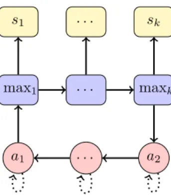
max1 . . . maxk
s1 . . . sk
a1 . . . a2
Figure 1: Illustration of Lemma 9: a1anda2are average fork vertices. Vertices on the top are MAX vertices, labelled from 1 tok, that lead to sinks. maxk is the last MAX vertex before a fork vertex. Assume it is optimal to open at least one MAX vertex. Then, the first open MAX vertex (wrt to the labelling) of the optimal strategy of the subgame open at maxk is open as well in the optimal strategy of the initial game.
The Lemma is illustrated on Figure 1.
Finally, if the optimal strategy is open at some MAX vertex, then the fol- lowing algorithm can be run to compute the values ofG:
1. Letxbe the last MAX vertex before some fork vertex, andσ1the partial strategy open at x. G[σ1] is an SSG that haska−1 fork vertices (recall that G is strongly connected). When solved, it provides a set S[σ1] of open MAX vertices. There are at mostka+ka−1 vertices that are the first in S[σ1] after a fork vertex. Then, from Lemma 9, it is optimal to open at least one of them inG.
2. For eachy that is the first in S[σ1] after a fork vertex:
(a) compute the values ofG[σ2],σ2 being the partial strategy open aty, (b) if local optimality condition is satisfied fory inG, return the values.
This algorithm computes at most 2kaSSGs withka−1 average fork vertices.
In the worst case, the same algorithm must be run for the MIN vertices. Using theorem 6 for the casekp=ka= 0, we obtain Theorem 3 and its corollary.
4 Feedback vertex set
A feedback vertex set is a set of vertices in a directed graph such that removing them yields a DAG. Computing a minimal vertex set is anNP-hard problem [10], but it can be solved with a FPT algorithm [5]. Assume the size of the minimal vertex set is fixed, we prove in this section that we can find the optimal strategies
in polynomial time. Remark that, to prove such a theorem, we cannot use the result on bounded number of cycles since a DAG plus one vertex may have an exponential number of cycles. Moreover a DAG plus one vertex may have a large number of positional vertices with several arcs in a cycle, thus we cannot use the algorithm to solve MAX-acyclic plus a few non acyclic MAX vertices.
The method we present works by transformingkvertices into sinks and could thus be used for other classes of SSGs. For instance, it could solve in polynomial time the value problem for games which are MAX-acyclic when k vertices are removed.
4.1 The dichotomy method
We assume from now on that all SSGs are stopping. In this subsection, we explain how to solve an SSG by solving it several times but with one vertex less.
First we remark that turning any vertex into a sink of its own value in the original game does not change any value.
Lemma 10. LetGbe an SSG andxone of its vertex. LetG′ be the same SSG asGexcept thatxhas been turned into a sink vertex of value ValG(x). For all verticesy, ValG(y) =ValG′(y).
Proof. The optimality condition of Theorem 1 are exactly the same in Gand G′. Since the game is stopping, there is one and only one solution to these equations and thus the values of the vertices are identical in both games.
The values in an SSG are monotone with regards to the values of the sinks, as proved in the next lemma.
Lemma 11. LetGbe an SSG and sone of its sink vertex. LetG′ be the same SSG as G except that the value of s has been increased. For all vertices x, ValG(x)≤ValG′(x).
Proof. Let fix a pair of strategy (σ, τ) and a vertexx. We have:
Val(σ,τ),G(x) = X
y∈VSIN K
P(x y) ValG(y)
Val(σ,τ),G(x)≤ X
y∈VSIN K
P(x y) ValG′(y) = Val(σ,τ),G′(x)
because ValG(x) = ValG′(x) except when x = s, ValG(s) ≤ ValG′(s). Since the inequality is true for every pair of strategies and every vertex, the lemma is proved.
Letxbe an arbitrary vertex ofGand letG[v] be the same SSG, except that xbecomes a SINK vertex of value v. We define the functionf by:
if x is a MAX vertex, f(v) = max{ValG[v](y) : (x, y)∈A} if x is a MIN vertex, f(v) = min{ValG[v](y) : (x, y)∈A} if x is an AVE vertex, f(v) =12ValG[v](x1) + ValG[v](x2)
Lemma 12. There is a uniquev0 such thatf(v0) =v0 which isv0=ValG(x).
Moreover, for allv > v0,f(v0)< v0 and for allv < v0,f(v0)> v0.
Proof. The local optimality conditions given in Theorem 1 are the same inGand G[v] except the equation f(ValG(x)) = ValG(x). Therefore, when f(v0) =v0, the values ofG[v] satisfy all the local optimality conditions ofG. Thusv0is the value ofsin G. Since the game is stopping there is at most one such value.
Conversely, letv0 be the value ofsinG. By Lemma 10, the values inG[v0] are the same as inGfor all vertices. Therefore the local optimality conditions inGcontains the equationf(v0) =v0.
We have seen that f(v) = v is true for exactly one value of v. Since the function f is increasing by Lemma 11 and because f(0)≥0 and f(1)≤1, we have for allv > v0, f(v0)< v0 and for allv < v0,f(v0)> v0.
The previous lemma allows to determine the value ofxinGby a dichotomic search by the following algorithm. We keep refining an interval [min, max]
which contains the value ofx, with starting valuesmin= 0 andmax= 1.
1. Whilemax−min≤6−na do:
(a) v= (min+max)/2 (b) Compute the values ofG[v]
(c) Iff(v)> v thenmin=v (d) Iff(v)< v thenmax=v
2. Return the unique rational in [min, max] of denominator less than 6−na2 Theorem 7. LetGbe an SSG withnvertices andxone of its vertex. Denote by C(n)the complexity to solveG[v], then we can compute the values ofGin time O(nC(n)). In particular an SSG which can be turned into a DAG by removing one vertex can be solved in timeO(n2).
Proof. Letv0 be the value of xin G, which exists since the game is stopping.
By Lemma 12 it is clear that the previous algorithm is such thatv0 is in the interval [min, max] at any time. Moreover, by Lemma 1 we know thatv0= ab whereb≤6na2 . At the end of the algorithm,max−min≤6−na therefore there is at most one rational of denominator less than 6na2 in this interval. It can be found exactly withO(na) arithmetic operations by doing a binary search in the Stern-Brocot tree (see for instance [12]).
One last call toG[v0] gives us all the exact values ofG. Since the algorithm stops whenmax−min≤6−na, we have at most O(na) calls to the algorithm solvingG[v]. All in all the complexity isO(naC(n) +na) that isO(naC(n)).
In the case where G[v] is an acyclic graph, we can solve it in linear time which gives us the stated complexity.
4.2 Feedback Vertex Set of Fixed Size
LetG be an SSG such that X is one of its minimal vertex feedback set. Let k=|X|. The game is assumed to be stopping. Since the classical transfor- mation [6] into a stopping game does not change the size of a minimal vertex feedback set, it will not change the polynomiality of the described algorithm.
However the transformation produces an SSG which is quadratically larger, thus a good way to improve the algorithm we present would be to relax the stopping assumption.
In this subsection we will consider games whose sinks have dyadic values, since they come from the dichotomy of the last subsection. The gcd of the values of the sinks will thus be the maximum of the denominators. The idea to solveGis to get rid of X, one vertex at a time by the previous technique.
The only thing we have to be careful about is the precision up to which we have to do the dichotomy, since each step adds a new sink whose value has a larger denominator.
Theorem 8. There is an algorithm which solves any stopping SSG in time O(nk+1)wherenis the number of vertices andkthe size of the minimal feedback vertex set.
Proof. First recall that we can find a minimal vertex with an FPT algorithm.
You can also check every set of sizek and test in linear time whether it is a feedback vertex set. Thus the complexity of finding such a set, that we denote byX ={x1, . . . , xk}, is at worstO(nk+1). Let denote byGithe gameGwhere x1 toxi has been turned into sinks of some values. If we want to make these values explicit we writeGi[v1, . . . , vi] wherev1tovi are the values of the sinks.
We now use the algorithm of Theorem 7 recursively, that is we apply it to re- duce the problem of solvingGi[v1, . . . , vi] to the problem of solvingGi+1[v1, . . . , vi, vi+1] for several values ofvi+1. SinceGk is acyclic, it can be solved in linear time. Therefore the only thing we have to evaluate is the number of calls to this last step. To do that we have to explain how precise should be the dichotomy to solveGi, which will give us the number of calls to solveGi in function of the number of calls to solveGi+1.
We prove by induction on ithat the algorithm, to solve Gi, makes log(pi) calls to solve Gi+1, where the value vi+1 is a dyadic number of numerator bounded by pi = 6(2i+1−1)na. Theorem 7 proves the casei = 0. Assume the property is proved fori−1, we prove it for i. By induction hypothesis, all the denominators ofv1, . . . , viare power of two and their gcd is bounded bypi. By Lemma 1, the value ofxi is a rational of the form ab whereb≤pi6na2 . We have to do the dichotomy up to the square of pi6na2 to recover the exact value of xi in the game Gi(v1, . . . , vi−1). Thus the bound on the denominator of vi+1
is pi+1 = p2i6na. That is pi+1 = 62(2i+1−1)na6na = 6(2i+2−1)na, which proves the induction hypothesis. Since we do a dichotomy up to a precisionpi+1, the number of calls is clearly log(pi+1).
In conclusion, the number of calls toGk is
k−1
Y
i=0
log(6(2i+1−1)na)≤2k2log(6)knka.
Since solving a gameGk can be done in linear time the total complexity is in O(nk+1).
Acknowledgements This research was supported by grant ANR 12 MONU- 0019 (project MARMOTE). Thanks to Yannis Juglaret for being so motivated to learn about SSGs and to Luca de Feo for insights on rationals and their representations.
References
[1] Daniel Andersson, Kristoffer Arnsfelt Hansen, Peter Bro Miltersen, and Troels Bjerre Sørensen. Deterministic graphical games revisited. InLogic and Theory of Algorithms, pages 1–10. Springer, 2008.
[2] Daniel Andersson and Peter Bro Miltersen. The complexity of solving stochastic games on graphs. In Algorithms and Computation, pages 112–
121. Springer, 2009.
[3] Dietmar Berwanger, Anuj Dawar, Paul Hunter, Stephan Kreutzer, and Jan Obdrˇz´alek. The dag-width of directed graphs. Journal of Combinatorial Theory, Series B, 102(4):900–923, 2012.
[4] Krishnendu Chatterjee and Nathana¨el Fijalkow. A reduction from parity games to simple stochastic games. In GandALF, pages 74–86, 2011.
[5] Jianer Chen, Yang Liu, Songjian Lu, Barry O’sullivan, and Igor Razgon.
A fixed-parameter algorithm for the directed feedback vertex set problem.
Journal of the ACM (JACM), 55(5):21, 2008.
[6] Anne Condon. The complexity of stochastic games.Information and Com- putation, 96(2):203–224, 1992.
[7] Anne Condon. On algorithms for simple stochastic games. Advances in computational complexity theory, 13:51–73, 1993.
[8] John Fearnley. Exponential lower bounds for policy iteration. pages 551–
562, 2010.
[9] Oliver Friedmann. An exponential lower bound for the parity game strategy improvement algorithm as we know it. InLogic In Computer Science, 2009.
LICS’09. 24th Annual IEEE Symposium on, pages 145–156. IEEE, 2009.
[10] Michael R Gary and David S Johnson. Computers and intractability: A guide to the theory of NP-completeness, 1979.
[11] Hugo Gimbert and Florian Horn. Simple stochastic games with few ran- dom vertices are easy to solve. In Foundations of Software Science and Computational Structures, pages 5–19. Springer, 2008.
[12] Knuth Graham and Donald E Knuth. Patashnik, concrete mathematics.
InA Foundation for Computer Science, 1989.
[13] Alan J Hoffman and Richard M Karp. On nonterminating stochastic games.
Management Science, 12(5):359–370, 1966.
[14] Yannis Juglaret. ´Etude des simple stochastic games.
[15] Walter Ludwig. A subexponential randomized algorithm for the simple stochastic game problem. Information and computation, 117(1):151–155, 1995.
[16] Jan Obdrˇz´alek. Clique-width and parity games. InComputer Science Logic, pages 54–68. Springer, 2007.
[17] Lloyd S Shapley. Stochastic games. Proceedings of the National Academy of Sciences of the United States of America, 39(10):1095, 1953.
[18] Colin Stirling. Bisimulation, modal logic and model checking games.Logic Journal of IGPL, 7(1):103–124, 1999.
[19] Rahul Tripathi, Elena Valkanova, and VS Anil Kumar. On strategy im- provement algorithms for simple stochastic games. Journal of Discrete Algorithms, 9(3):263–278, 2011.