HAL Id: hal-03517003
https://hal.inria.fr/hal-03517003
Submitted on 7 Jan 2022
HAL is a multi-disciplinary open access archive for the deposit and dissemination of sci- entific research documents, whether they are pub- lished or not. The documents may come from teaching and research institutions in France or abroad, or from public or private research centers.
L’archive ouverte pluridisciplinaire HAL, est destinée au dépôt et à la diffusion de documents scientifiques de niveau recherche, publiés ou non, émanant des établissements d’enseignement et de recherche français ou étrangers, des laboratoires publics ou privés.
Assia Mahboubi, Thomas Sibut-Pinote
To cite this version:
Assia Mahboubi, Thomas Sibut-Pinote. A formal proof of the irrationality of ζ(3). Logical Meth- ods in Computer Science, Logical Methods in Computer Science Association, 2021, 17 (1), pp.1-25.
�10.23638/LMCS-17(1:16)2021�. �hal-03517003�
A FORMAL PROOF OF THE IRRATIONALITY OF ζ(3)
ASSIA MAHBOUBI AND THOMAS SIBUT-PINOTE
LS2N UFR Sciences et Techniques, 2 rue de la Houssini`ere, BP 92208 44322 Nantes Cedex 3 France e-mail address: Assia.Mahboubi@inria.fr
e-mail address: thomas.sibut-pinote@ens-lyon.org
Abstract. This paper presents a complete formal verification of a proof that the evaluation of the Riemann zeta function at 3 is irrational, using theCoqproof assistant. This result was first presented by Ap´ery in 1978, and the proof we have formalized essentially follows the path of his original presentation. The crux of this proof is to establish that some sequences satisfy a common recurrence. We formally prove this result by ana posteriori verification of calculations performed by computer algebra algorithms in a Maple session.
The rest of the proof combines arithmetical ingredients and asymptotic analysis, which we conduct by extending theMathematical Componentslibraries.
1. Introduction In 1978, Ap´ery proved thatζ(3), which is the sumP∞
i=1 1
i3 now known as theAp´ery constant, is irrational. This result was the first dent in the problem of the irrationality of the evaluation of the Riemann zeta function at odd positive integers. As of today, this problem remains a long-standing challenge of number theory. Zudilin [Zud01] showed that at least one of the numbersζ(5),ζ(7),ζ(9), ζ(11) must be irrational. Ball and Rivoal [Riv00, BR01] established that there are infinitely many irrational odd zeta values. Fischler, Sprang and Zudilin proved [FSZ19] that there are asymptotically more than any power of log(s) irrational values of the Riemann zeta function at odd integers between 3 and s. But today ζ(3) is the only known such value to be irrational.
Van der Poorten reports [vdP79] that Ap´ery’s announcement of this result was at first met with wide skepticism. His obscure presentation featured “a sequence of unlikely assertions” without proofs, not the least of which was an enigmatic recurrence (Lemma 3.3) satisfied by two sequences aand b. It took two months of collaboration between Cohen, Lenstra, and Van der Poorten, with the help of Zagier, to obtain a thorough proof of Ap´ery’s theorem:
Theorem 1.1 (Ap´ery, 1978). The constant ζ(3) is irrational.
Key words and phrases: formal proof, number theory, irrationality, creative telescoping, symbolic compu- tation, Coq, Ap´ery’s recurrences, Riemann zeta function.
This work was supported in part by the project FastRelax ANR-14-CE25-0018-01.
LOGICAL METHODS
l
IN COMPUTER SCIENCE DOI:10.23638/LMCS-17(1:16)2021© A. Mahboubi and T. Sibut-Pinote CC Creative Commons
In the present paper, we describe a formal proof of this theorem inside the Coq proof assistant [The20], using the Mathematical Components libraries [coq19]. This formalization follows the structure of Ap´ery’s original proof. However, we replace the manual verification of recurrence relations by an automatic discovery of these equations, using symbolic computation. For this purpose, we use Maple packages to perform calculations outside the proof assistant, and we verify a posteriori the resulting claims inside Coq. By combining these verified results with additional formal developments, we obtain a complete formal proof of Theorem 1.1, formalized using theCoqproof assistant without additional axiom. In particular, the proof is entirely constructive, and does not rely on the axiomatic definition of real numbers provided inCoq’s standard library. A previous paper [CMSPT14]
reported on the implementation of the cooperation between a computer algebra system and a proof assistant used in the formalization. The present paper is self-contained: it includes a summary of the latter report, and provides more details about the rest of the formal proof.
In particular, it describes the formalization of an upper bound on the asymptotic behavior of lcm(1, ..., n), the least common multiple of the integers from 1 to n, a part of the proof which was missing in the previous report.
The rest of the paper is organized as follows. We first describe the background formal theories used in our development (Section 2). We then outline the proof of Theorem 1.1 (Section 3). We summarize the algorithms used in the Maple session, the data this session produces and the way this data can be used in formal proofs (Section 4). We then describe the proof of the consequences of Ap´ery’s recurrence (Section 5). Finally, we present an elementary proof of the bound on the asymptotic behavior of the sequence lcm(1, ..., n), which is used in this irrationality proof (Section 6), before commenting on related work and concluding (Section 7).
The companion code to the present article can be found in the following repository:
https://github.com/math-comp/apery.
2. Preliminaries
This section provides some hints about the representation of the different natures of numbers at stake in this proof in the libraries backing our formal development. It also describes a few extensions we devised for these libraries and sets some notations used throughout this paper. Most of the material presented here is related to the Mathematical Components libraries [coq19, GAA+13].
2.1. Integers. InCoq, the setNof natural numbers is usually represented by the typenat:
Inductive nat := O | S : nat → nat.
This type is defined in a prelude library, which is automatically imported by anyCoqsession.
It models the elements ofN using a unary representation: Coq’s parser reads the number 2 as the term S (S O). The structural induction principle associated with this inductive type coincides with the usual recurrence scheme on natural numbers. This is convenient for defining elementary functions on natural numbers, like comparison or arithmetical operations, and for developing their associated theory. However, the resulting programs are usually very naive and inefficient implementations, which should only be evaluated for the purpose of small scale computations.
The setZof integers can be represented by gluing together two copies of typenat, which provides a signed unary representation of integers:
Inductive int : Set := Posz of nat | Negz of nat.
If the term n : nat represents the natural number n ∈ N, then the term (Posz n): int
represents the integern∈Zand the term(Negz n): int represents the integer−(n+ 1)∈Z. In particular, the constructorPosz : nat → intimplements the embedding of type natinto type int, which is invisible on paper because it is just the inclusion N ⊂ Z. In order to mimic the mathematical practice, the constantPosz is declared as a coercion, which means in particular that unless otherwise specified, this function is hidden from the terms displayed by Coqto the user (in the current goal, in answers to search queries, etc).
TheMathematical Componentslibraries provide formal definitions of a few elemen- tary concepts and results from number theory, defined on the type nat. For instance, they provide the theory of Euclidean division, a boolean primality test, the elementary properties of the factorial function, of binomial coefficients, etc. In the rest of the paper, we use the standard mathematical notationsn! and mn
for the corresponding formal definition of the factorial and of the binomial coefficients respectively. These libraries also define thep-adic valuationvp(n) of a number n: if p is a prime number, it is the exponent ofp in the prime decomposition ofn. However, we had to extend the available basic formal theory with a few extra standard results, like the formula giving thep-adic valuation of factorials:
Lemma 2.1. For any n∈N and for any prime number p:
vp(n!) =
blogpnc X
i=1
n pi
.
Incidentally, the formal version of this formula is a typical example of the slight variations one may introduce in a mathematical statement, in order to come up with a formal sentence which is not only correct and faithful to the original mathematical result, but also a tool which is easy to use in subsequent formal proofs. First, although the fraction in the original statement of Lemma 2.1 may suggest that rational numbers play a role here, n
m
is in fact exactly the quotient of the Euclidean division ofn bym. In the rest of the paper, for n, m∈N andm non-zero, we thus writen
m
for the quotient of the Euclidean division ofn bym. Perhaps more interestingly, the formal statement of Lemma 2.1 rather corresponds to the following variant:
For any prime p and anyj, n∈N, such thatn < pj+1, vp(n!) =
j
X
i=1
n pi
.
Adding an extra variable to generalize the upper bound of the sum is a better option because it will ease unification when this formula is applied or used for rewriting. Moreover, we do not really need to introduce logarithms here: indeed,
logpn
is used to denote the largest power ofpsmaller thann. For this purpose, we could use the functiontrunc_log : nat → nat → nat
provided by the Mathematical Components libraries, which computes the greatest exponentα such that nα ≤m, in other words blognmc. Better yet, since the summand is zero when the index iexceeds this value, we can simplify the side condition on the extra variable and require only thatn < pj+1.
The basic theory of binomial coefficients present in theMathematical Components libraries describes their role in elementary enumerative combinatorics. However, when
viewing binomial coefficients as a sequence which is a certain solution of a recurrence system, it becomes natural to extend their domain of definition to integers: we thus developed a small library about these generalized binomial coefficients. We also needed to extend these libraries with properties of multinomial coefficients. For n, k1, . . . , kl∈N, with k1+· · ·+kl=n, the coefficient of xk11· · ·xkll in the formal expansion of (x1+· · ·+xl)n is called a multinomial coefficient and denoted k n
1,...,kl
. Its value is k n!
1!...kl! or equivalently,
l
Q
i=1
k1+···+ki
ki
. The latter formula provides for free the fact that multinomial coefficients are non-negative integers and we use it in our formal definition: for(l : seq nat) a finite sequencel1, . . . , ls of natural numbers, then(multinomial l) is the multinomial coefficient l1l+···+ls
1,...,ls
:
Definition multinomial (l : seq nat) : nat :=
\prod_(0 ≤ i < size l) (binomial (\sum_(0 ≤ j < i.+1) l‘_j) l‘_i).
From this definition, we prove formally the other characterizations, as well as the generalized Newton formula describing the expansion of (x1+· · ·+xl)n.
2.2. Rational numbers, algebraic numbers, real numbers. In the Mathematical Components libraries, rational numbers are represented using a dependent pair. This type construct, also called Σ-type, is specific to dependent type theory: it makes possible to define a type that decorates a data with a proof that a certain property holds on this data. The Mathematical Componentslibraries also include a construction of the algebraic closure for countable fields, and thus a construction ofQ, algebraic closure of Q, the field of rational numbers. The corresponding type, namedalgC is equipped with a structure of (partially) ordered, algebraically closed field [GAA+13]. Slightly abusing notation, we denote byQ∩R the subset of Qcontaining elements with a zero imaginary part and we call such elements real algebraic numbers.
Almost all the irrational numbers involved in the present proof are real algebraic numbers, and more precisely, they are of the formrn1 forr a non-negative rational number r and for n∈N. The only place where these numbers play a role is in auxiliary lemmas for the proof of the asymptotic behavior of the sequence (`n)n∈N, where`n is the least common multiple of integers between 1 and n. They appear in inequalities expressing signs and estimations.
It might come as a surprise that we used the type algCof algebraic (complex) numbers to cast these quantities, although we do not actually need imaginary complex numbers. But this choice proved convenient due to the fact that the typealgC features both a definition of n-th roots, and a clever choice of partial order. Indeed, althoughQcannot be ordered as a field, it is equipped with a binary relation, denoted ≤, which coincides with the real order relation on Q∩R:
∀x, y∈Q, x≤y⇔y−x∈R≥0. In particular, for anyz∈Q:
0≤z⇔z∈R≥0 andz≤0⇔z∈R≤0.
Moreover, the typealgC is equipped with a function n.-root : algC → algC, defined for any
(n : nat), such that(n.-root z) is then-th (complex) root of z with minimal non-negative argument. Crucially, when(z : algC) represents a non-negative real number, (n.-root z)
coincides with the definition of the real n-th root, and thus the following equivalence holds:
Lemma rootC_ge0 (n : nat) (z : algC) : n > 0 → (0 ≤ n.-root z) = (0 ≤ z).
The shape of Lemma rootC_ge0 is typical of the style pervasive in the Mathematical Components libraries, where equivalences between decidable statements are stated as boolean equalities. It expresses that for an algebraic numberx, that is forx∈Q, we have xn1 ∈R≥0 if and only if x∈R≥0.
The one notable place at which we need to resort to a larger subset of the real numbers is the definition of the numberζ(3), if only because as of today, it is not even known whether ζ(3) is algebraic or transcendental. This number is actually defined as the limit of the partial sumsPn
m=1 1
m3, so we start our formal study by establishing the existence of this limit.
More precisely, we show that this sequence of partial sums is aCauchy sequence, with an explicit modulus of convergence.
Definition 2.2. ACauchy sequence is a sequence (xn)n∈N∈QN together with a modulus of convergence mx : Q→ N such that if ε is a positive rational number, then any two elements of index greater thanmx(ε) are separated at most byε.
Proposition 2.3. The sequence zn=Pn m=1
1
m3 is a Cauchy sequence.
Two sequencesxandyareCauchy equivalent ifxandyare both Cauchy sequences, and if eventually |xn−yn|< ε, for any ε >0. Real numbers could be constructed formally by introducing a quotient type, whose element are the equivalent classes of the latter relation.
But this is rather irrelevant for this formalization, which involves explicit sequences and their asymptotic properties, rather than real numbers. For this reason, the formal statements in this formal proof only involve sequences of rational numbers, and a type of Cauchy sequences which pairs such a sequence with a proof that it has the Cauchy property. For instance, for two Cauchy sequencesx andy, we writex < y if there is a rational numberε >0 such that eventuallyxn+ε≤yn.
We benefited from the formal library about Cauchy sequences developed by Co- hen [Coh12]. This library defines Cauchy sequences of elements in a totally ordered field, and introduces a type(creal F) of Cauchy sequences over the totally ordered field F, given as a parameter. We thus use the instance(creal rat). The infix notation ==, in the notation scope CR, denotes the equivalence of Cauchy sequences, as in the statement (x == y)%CR, which states that the two Cauchy sequencesx, y are equivalent. The library implements a setoid of field operations over this type [BCP03, Soz09], so as to facilitate substitutions for equivalents in formulas. In addition, the library provides a tactic called bigenough, which eases formal proofs by allowing a dose of laziness. This tactic is specially useful in proofs that a certain property on sequences is eventually true, which involve constructing effective moduli of convergence.
The formal statement corresponding to Theorem 1.1 is thus:
Theorem zeta_3_irrational : ~ ∃(r : rat), (z3 == r%:CR)%CR.
where the postfix notation r%:CR denotes the Cauchy sequence whose elements are all equal to the rational number(r : rat). The term z3is the Cauchy sequence corresponding to the partial sums (zn)n∈N, that is, the dependent pair of this sequence with a proof of Property 2.3.
The formal statement thus expresses that no constant rational sequence can be Cauchy equivalent to (zn)n∈N. Interestingly, a long-lasting typo has marred the formal statement of theorem zeta_3_irrationalin the corresponding Coq libraries, until writing the revised version of the present paper. Until then, the (inaccurate) statement was indeed:
Theorem incorrect_zeta_3_irrational : ~ ∃(r : rat), (z3 = r%:CR)%CR.
Replacing== by =changes the statement completely, as it now expresses that there is no constant sequence of rationals equal to z3: and this is trivially true. The typo was already present in the version of the code that we made public for our previous report [CMSPT14], and the typo has remained unnoticed since. Yet fortunately, theproof script was right, and actually described a correct proof of the stronger statementzeta_3_irrational.
2.3. Notations. In this section, we provide a few hints on the notations used in the formal statements corresponding to the paper proof, so as to make precise the meaning of the statements we have proved formally. Indeed, this development makes heavy use of the notation facilities offered by the Coq proof assistant, so as to improve the readability of formulas. For instance, notation scopes allow to use the same infix notation for a relation on type nat, and in this case(x < y) unfolds to(ltn x y): bool, or for a relation on typecreal rat), and in that case(x < y) unfolds to(lt_creal x y): Prop, the comparison predicate described in Section 2.2. Notation scopes can be made explicit using post-fixed tags: (x < y)%N is interpreted in the scope associated with natural numbers, and(x < y)%CR, in the scope associated with Cauchy sequences.
Generic notations can also be shared thanks to type-class like mechanisms. The Math- ematical Componentslibraries feature a hierarchy of algebraic structures [GGMR09], which organizes a corpus of theories and notations shared by all the instances of a same structure. This hierarchy implements inheritance and sharing using Coq’s mechanisms of coercions and of canonical structures [MT13]. Each structure in the hierarchy is modeled by a dependent record, which packages a type with some operations on this type and with requirements on these operations. In order to equip a given type with a certain structure, one has to endow this type with enough operations and properties, following the signature prescribed by the structure. For example, these structures are all discrete, which means that they require a boolean equality test. In turn, all instances of all these structures share the same infix notation(x == y) for the latter boolean equality test betweenx and y: this notation makes sense forx,y in type nat,int,rat, alC, etc. because all these types are instances of the same structure. For instance, although typerat is a dependent pair (see Section 2.2), the boolean comparison test only needs to work with the data: by Hedberg’s theorem [Hed98], the proof stored in the proof component can be made irrelevant. Note that the situation is different for the type(creal rat) of Cauchy sequences. The formal statement of theoremzeta_3_irrational(see Section 2.2) uses the same==infix symbol, but in a different scope, in which it refers toProp-valued Cauchy equivalence. Indeed, this relation cannot be turned constructively into a boolean predicate, as the comparison of Cauchy sequences is not effective. The typealgC of algebraic numbers by contrast enjoys the generic version of the notation, as ordered fields only require a partial order relation.
Partial order, but also units of a ring, and inverse operations are examples of operations involved in some structures of the hierarchy, that make sense only on a subset of the elements of the carrier. In the dependent type theory implemented byCoq, it would be possible to use a dependent pair in order to model the source type of such an inverse operation. Instead, as a rule of thumb, the signature of a given structure avoids using rich types as the source types of their operations but rather “curry” the specification. For instance, the source type of the inverse operation in the structure of ring with units is the carrier type itself, but the signature of this structure also has a boolean predicate, which selects the units in this carrier type. The inverse operation has a default behavior outside units and the equations of the theory that involve inverses are typically guarded with invertibility conditions. Hence
although the expressionx^-1 * x is syntactically well-formed for any termx of an instance of ring with units, it can be rewritten to1 only whenx is known to be invertible.
The readability of formulas also requires dealing in a satisfactory manner with the inclusion of the various collections of numbers at stake, that are represented with distinct types, for instance:
N⊂Z⊂Q⊂Q.
The implementation of the inclusionN⊂Zwas mentioned in Section 2.1. The canonical embedding of typeint is available in the generic theory of rings, but unfortunately, it cannot be declared as a coercion, and eluded in formal statements: the type of the corresponding constant would violate the uniform inheritance condition prescribed by Coq’s coercion mechanism [The20]. Its formal definition hence comes with a generic postfix notation_%:~R, modeled as a reminiscence of the syntax of notation scopes and used to cast an integer as an element of another ring. The latter embedding is pervasive in formulas expressing the recurrence relations involved in this proof. Indeed, these recurrence relations feature polynomial coefficients in their indices and relate the rational elements of their solutions.
See for instance Equation 3.2.
2.4. Computations. Using the unary representation of integers described in Section 2.1, the command:
Compute 100*1000.
which asks Coq to evaluate this product, triggers a stack overflow. For the purpose of running computations insideCoq’s logic, on integers of a medium size, an alternate data- structure is required, together with less naive implementations of the arithmetical operations.
The present formal proof requires this nature of computations at several places, for instance in order to evaluate sequences defined by a recurrence relation at a few particular values.
For these computations, we used the binary representation of integers provided by the
ZArith library included in the standard distribution ofCoq, together with the fast reduction mechanism included in Coq’s kernel [GL02].
These two ingredients are also used behind the scene by tactics implementing verified decision procedures. For instance, we make extensive use of proof commands dedicated to the normalization of algebraic expressions like thefield tactic for rational fractions, and the
ring tactic for polynomials [GM05]. The field tactic generates proof obligations describing sufficient conditions for the simplifications it made. In our case, these conditions in turn are solved using thelia decision procedure for linear arithmetics [Bes07].
These tactics work by first converting formulas in the goal into instances of appropriate data structures, suitable for larger scale computation. This pre-processing, hidden to the user, is performed by extra-logical code that is part of the internal implementation of these tactics. The situation is different when a computational step in a proof requires the evaluation of a formula at a given argument, and when both the formula and the argument are described using proof-oriented, inefficient representations. In that case, for instance for evaluating terms in a given sequence, we used the CoqEAL library [CDM13], which provides an infrastructure automating the conversion between different data-structures and algorithms used to model the same mathematical objects, like different representations of integers or different implementations of a matrix product. Note that although the CoqEAL library itself depends on a library for big numbers, which provides direct access in Coq
toOcaml’s library for arbitrary-precision, arbitrary-size signed integers, the present proof does not need this feature.
3. Outline of the proof
There exists several other proofs of Ap´ery’s theorem. Notably, Beukers [Beu79] published an elegant proof, based on integrals of pseudo-Lengendre polynomials, shortly after Ap´ery’s announcement. According to Fischler’s survey [Fis04], all these proofs share a common structure. They rely on the asymptotic behavior of the sequence `n, the least common multiple of integers between 1 and n, and they proceed by exhibiting two sequences of rational numbersan andbn, which have the following properties:
(1) For a sufficiently largen:
an∈Z and 2`3nbn∈Z; (2) The sequence δn=anζ(3)−bn is such that:
lim sup
n→∞
|2δn|n1 ≤(√
2−1)4; (3) For an infinite number of values n,δn6= 0.
Altogether, these properties entail the irrationality of ζ(3). Indeed, if we suppose that there existsp, q∈Zsuch that ζ(3) = pq, then 2q`3nδn is an integer whenn is large enough. One variant of the Prime Number theorem states that`n=en(1+o(1)) and since (√
2−1)4e3 <1, the sequence 2q`3nδn has a zero limit, which contradicts the third property. Actually, the Prime Number theorem can be replaced by a weaker estimation of the asymptotic behavior of `n, that can be obtained by more elementary means.
Lemma 3.1. Let `n be the least common multiple of integers1, . . . , n, then
`n=O(3n).
Since we still have (√
2−1)433 < 1, this observation [Han72, Fen05] is enough to conclude. Section 6 discusses the formal proof of Lemma 3.1, an ingredient which was missing at the time of writing the previous report on this work [CMSPT14].
In our formal proof, we consider the pair of sequences proposed by Ap´ery in his proof [Ap´e79, vdP79]:
an=
n
X
k=0 n k
2 n+k k
2
, bn=anzn+
n
X
k=1 k
X
m=1
(−1)m+1 nk2 n+k k
2
2m3 mn n+m
m
(3.1)
where zn denotesPn m=1 1
m3, as already used in Proposition 2.3.
By definition,an is a positive integer for any n∈N. The integrality of 2`3nbnis not as straightforward, but rather easy to see as well: each summand in the double sum defining bn has a denominator that divides 2`3n. Indeed, after a suitable re-organization in the expression of the summand, using standard properties of binomial coefficients, this follows easily from the following slightly less standard property:
Lemma 3.2. For any integers i, j, n such that 1≤j≤i≤n, j ji
divides`n.
Proof. Fori, j, n such that 1≤j≤i≤n, the proof goes by showing that for any primep, the p-adic valuation of j ji
is at most that of `n. Let us fix a prime number p. Let tp(i) be the largest integer e such that pe ≤ i. By definition, and since i ≤ n, we thus have ptp(i)|`n and sotp(i)≤vp(`n). Hence it suffices to prove that vp( ij
)≤tp(i)−vp(j). Using Lemma 2.1, and because j≤i < ptp(i)+1, we have:
vp( i
j
) =
tp(i)
X
k=1
i pk
−(
tp(i)
X
k=1
j pk
+
tp(i)
X
k=1
(i−j) pk
) Remember that for a, b∈N, a
b
is just amodulo b. Now for 1≤k≤vp(j), and because pk|j, we have j
i pk
k
=j
j pk
k
+j(i−j)
pk
k
, and thus:
vp( i
j
) =
tp(i)
X
k=vp(j)+1
i pk
−(
tp(i)
X
k=vp(j)+1
j pk
+
tp(i)
X
k=vp(j)+1
(i−j) pk
)
=
tp(i)−vp(j)
X
k=1
i pvp(j)+k
−(
tp(i)−vp(j)
X
k=1
j pvp(j)+k
+
tp(i)−vp(j)
X
k=1
(i−j) pvp(j)+k
) Now for any 1≤k≤tp(i)−vp(j), we have:
i pvp(j)+k
≤ j
pvp(j)+k
+
(i−j) pvp(j)+k
+ 1
Summing both sides fork from 1 totp(i)−vp(j) and using the previous identity forvp( ji ) eventually proves thatvp( ji
)≤tp(i)−vp(j), which concludes the proof.
The rest of the proof is a study of the sequenceδn=anζ(3)−bn. It not difficult to see that δn tends to zero, from the formulas defining the sequencesaandb, but we also need to prove that it does so fast enough to compensate for`3n, while being positive. In his original proof, Ap´ery derived the latter facts by combining the definitions of the sequencesaand b with the study of a mysterious recurrence relation. Indeed, he made the surprising claim that Lemma 3.3 holds:
Lemma 3.3. For n≥0, the sequences (an)n∈N and (bn)n∈N satisfy the same second-order recurrence:
(n+ 2)3yn+2−(17n2+ 51n+ 39)(2n+ 3)yn+1+ (n+ 1)3yn= 0. (3.2) Equation 3.2 is a typical example of a linear recurrence equation with polynomial coefficients and standard techniques [Sal03, vdP79] can be used to study the asymptotic behavior of its solutions. Using this recurrence and the initial conditions satisfied by a and b, one can thus obtain the two last properties of our criterion, and conclude with the irrationality of ζ(3). For the purpose of our formal proof, we devised an elementary version of this asymptotic study, mostly based on variations on the presentation of van der Poorten [vdP79]. We detail this part of the proof in Section 5.
Using only Equation 3.2, even with sufficiently many initial conditions, it would not be easy to obtain the first property of our criterion, about the integrality of an and bn for a large enough n. In fact, it would also be difficult to prove that the sequenceδ tends to zero:
we would only know that it has a finite limit, and how fast the convergence is. By contrast, it is fairly easy to obtain these facts from the explicit closed forms given in Formula 3.1.
The proof of Lemma 3.3 was by far the most difficult part in Ap´ery’s original exposition.
In his report [vdP79], van der Poorten describes how he, with other colleagues, devoted significant efforts to this verification after having attended the talk in which Ap´ery exposed his result for the first time. Actually, the proof of Lemma 3.3 boils down to a routine calculation using the two auxiliary sequencesUn,k and Vn,k, themselves defined in terms of λn,k= nk2 n+k
k
2
(with λn,k = 0 if k <0 ork > n):
Un,k = 4(2n+ 1)(k(2k+ 1)−(2n+ 1)2)λn,k, Vn,k = Un,k
n
X
m=1
1 m3 +
k
X
m=1
(−1)m−1 2m3 mn n+m
m
!
+5(2n+ 1)k(−1)k−1 n(n+ 1)
n k
n+k k
The key idea is to compute telescoping sums for U and V. For instance, we have:
Un,k−Un,k−1 = (n+ 1)3λn+1,k−(34n3+ 51n2+ 27n+ 5)λn,k+n3λn−1,k (3.3) Summing Equation 3.3 on kshows that the sequence asatisfies the recurrence relation of Lemma 3.3. A similar calculation proves the analogue forb, using telescoping sums of the sequence V.
Not only is the statement of Formula 3.2 difficult to discover: even when this recurrence is given, finding the suitable auxiliary sequences U and V by hand is a difficult task.
Moreover, there is no other known way of proving Lemma 3.3 than by exhibiting this nature of certificates. Fortunately, the sequences aandb belong in fact to a class of objects well known in the fields of combinatorics and of computer-algebra. Following seminal work of Zeilberger’s [Zei90], algorithms have been designed and implemented in computer-algebra systems, which are able to obtain linear recurrences for these sequences. For instance the Maple package Mgfun (distributed as part of the Algolib [alg13] library) implements these algorithms, among others. Basing on this implementation, Salvy wrote a Maple worksheet [Sal03] that follows Ap´ery’s original method but interlaces Maple calculations with human-written parts. In particular, this worksheet illustrates how parts of this proof, including the discovery of Ap´ery’s mysterious recurrence, can be performed by symbolic computations. Our formal proof of Lemma 3.3 follows an approach similar to the one of Salvy. It is based on calculations performed using the Algolib library, and certified a posteriori. This part of the formal proof is discussed in Section 4.1.
4. Algorithms, Recurrences and Formal Proofs
This section quotes and summarizes an earlier publication [CMSPT14], describing a joint work with Chyzak and Tassi.
Lemma 3.3 is the bottleneck in Ap´ery’s proof. Both sums an and bn in there are instances ofparameterized summation: they follow the pattern Fn=Pβ(n)
k=α(n)fn,k in which the summand fn,k, potentially the bounds, and thus the sum, depend on a parameter n.
This makes it appealing to resort to the algorithmic paradigm of creative telescoping, which was developed for this situation in computer algebra.
4.1. Recurrences as a data structure for sequences. A fruitful idea from the realm of computer algebra is to represent sequences not explicitly, such as the univariate (n!)n
or the bivariate ( nk
)n,k, but by a system of linear recurrences of which they are solutions such as{un+1 = (n+ 1)un}or{un+1,k = n+1−kn+1 un,k, un,k+1 = n−kk+1un,k}, accompanied with sufficient initial conditions. Sequences which can be represented in such a way are called
∂-finite. The finiteness property of their definition makes algorithmic most operations under which the class of∂-finite sequences is stable.
In the specific bivariate case which interests us, letSnbe the shift operator innmapping a sequence (un,k)n,k to (un+1,k)n,k and similarly, letSk map (un,k)n,k to (un,k+1)n,k. Linear recurrences canceling a sequencef can be seen as elements of a non-commutative ring of polynomials with coefficients in Q(n, k), and with the two indeterminatesSnand Sk, with the action (P ·f)n,k=P
(i,j)∈Ipi,j(n, k)fn+i,k+j, where subscripts denote evaluation. For example for fn,k= nk
, the previous recurrences once rewritten as equalities to zero can be represented asP ·f = 0 for P =Sn−n+1−kn+1 and P =Sk−n−kk+1, respectively.
Computer algebra gives us algorithms to produce canceling operators for operations such as the addition or product of two ∂-finite sequences, using for both its inputs and output a Gr¨obner basis as a canonical way to represent the set of their canceling operators, which gives some uniqueness guarantees.
The case of summing a sequence (fn,k) into a parameterized sum Fn = Pn
k=0fn,k is more involved: it follows the method of creative telescoping [Zei91], in two stages. First, an algorithmic step determines pairs (P, Q) satisfying
P ·f = (Sk−1)Q·f (4.1)
with P ∈Q(n)[Sn] and Q∈ A. To continue with our examplefn,k= nk
, we could choose P =Sn−2 and Q=Sn−1. Second, asystematic but not fully algorithmic step follows:
summing (4.1) fork between 0 and n+ degP yields
(P ·F)n= (Q·f)k=n+degP+1−(Q·f)k=0. (4.2) Continuing with our binomial example, summing (4.1) for k from 0 to n+ 1 (and taking special values into account) yieldsPn+1
k=0 n+1
k
−2Pn k=0
n k
= 0, a special form of (4.2) with right-hand side canceling to zero. This tells us that the sequence (Pn
k=0 n k
)n∈Nis a solution of the same recurrenceP =Sn−2 as (2n)n∈N: a simple check of initial values gives us the identity∀n∈N,2n=Pn
k=0 n k
. The formula (4.2) in fact assumes several hypotheses that hold not so often in practice; this will be formalized by Equation (4.3) below.
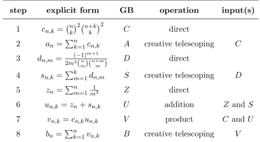
4.2. Ap´ery’s sequences are ∂-finite constructions. The sequencesaandbin (3.1) are
∂-finite: they have been announced to be solutions of (3.2). But more precisely, they can be viewed as constructed from “atomic” sequences by operations under which the class of ∂-finite sequences is stable. This is summarized in Table 1.
In this table, Gr¨obner bases are systems of recurrence operators: at each line in the table, the sequence given in explicit form is a solution of the system of recurrences described by the operators in the Gr¨obner basis column. Note that in fact none of these results rely on thespecific sequences in the explicit form: at each step, a new Gr¨obner basis is obtained from known ones, the ones that are cited in the input column. The table can also be read bottom-up for the purpose of verification: the Gr¨obner basis obtained at a given step can be verified usingonly the Gr¨obner bases obtained at some previous steps, all the way down toC and D. These operators describe a more general class of (germs of) sequences than
step explicit form GB operation input(s) 1 cn,k= nk2 n+k
k
2
C direct
2 an=Pn
k=1cn,k A creative telescoping C 3 dn,m= (−1)m+1
2m3(mn)(n+mm ) D direct 4 sn,k =Pk
m=1dn,m S creative telescoping D 5 zn=Pn
m=1 1
m3 Z direct
6 un,k=zn+sn,k U addition Z and S
7 vn,k =cn,kun,k V product C and U
8 bn=Pn
k=1vn,k B creative telescoping V
Table 1: Construction ofan andbn: At each step, the Gr¨obner basis named in column GB, which annihilates the sequence given in explicit form, is obtained by the corre- sponding operation on ideals, with input(s) given on the last column.
just the explicit sequences used in this table, thus initial conditions are needed to describe a precise sequence.
4.3. Provisos and sound creative telescoping. We illustrate the process of verifying candidate new recurrences using known ones on the example of Pascal’s triangle rule. One can “almost prove” Pascal’s triangle rule using only the following recurrences, satisfied by binomial coefficients:
un+1,k = n+ 1
n+ 1−kun,k and un,k+1 = n−k k+ 1un,k. Indeed, we have:
n+ 1 k+ 1
− n
k+ 1
− n
k
=
n+ 1 n−k
n−k
k+ 1 −n−k
k+ 1 −1 n k
= 0× n
k
= 0, but this requiresk6=−1 and k6=n. Therefore, this does not prove Pascal’s rule for alln and k. The phenomenon is general: computer algebra is unable to take denominators into account. This incomplete modeling of sequences by algebraic objects may cast doubt on these computer-algebra proofs, in particular when it comes to the output of creative-telescoping algorithms.
By contrast, in our formal proofs, we augmented the recurrences with provisos that restrict their applicability. In this setting, we validate a candidate identity like the Pascal triangle rule by a normalization modulo the elements of a Gr¨obner basis plus a verification that this normalization only involves legal instances of the recurrences. In the case of creative telescoping, Eq. (4.1) takes the form:
(n, k)∈/ ∆⇒(P·f,k)n= (Q·f)n,k+1−(Q·f)n,k, (4.3) where ∆⊂Z2 guards the relation and wheref,j denotes the univariate sequence obtained by specializing the second argument of f to j. Thus our formal analogue of Eq. (4.2) takes
this restriction into account and has the shape (P·F)n=
(Q·f)n,n+β+1−(Q·f)n,α
+
r
X
i=1 i
X
j=1
pi(n)fn+i,n+β+j
+ X
α≤k≤n+β ∧ (n,k)∈∆
(P ·f,k)n−(Q·f)n,k+1+ (Q·f)n,k,
(4.4)
forF the sequence with general term Fn=Pn+β
k=αfn,k and where P =
r
P
i=0
pi(n)Sni.
The last term of the right-hand side, which we will call the singular part, witnesses the possible partial domain of validity of relation (4.3). Thus the operator P is a valid recurrence for the sequence F if the right-hand side of Eq. (4.4) normalizes to zero, at least outside of an algebraic locus that will guard the recurrence.
4.4. Generated Operators, hand-written provisos, and formal proofs. For each step in Table 1, we make use of the data computed by the Maple session in a systematic way, using pretty-printing code to express this data in Coq. As mentioned in Section 4.3, we manually annotate each operator produced by the computer-algebra program with provisos and turn it this way into a conditional recurrence predicate on sequences. In our formal proof, each step in Table 1 consists in proving that some conditional recurrences on a composed sequence can be proved from some conditional recurrences known for the arguments of the operation.
These steps are far from automatic, mainly because the singular part yields terms which have to be reduced manually through trial-and-error using a Gr¨obner basis of annihilators for f, but also because we have to show that some rational-function coefficients of the remaining instances of f are zero. This is done through a combination of the field and lia proof commands, helped by some factoring of denominators pre-obtained in Maple.
4.5. Composing closures and reducing the order ofB. In order to complete the formal proof of Lemma 3.3, we verify formally that each sequence involved in the construction ofan and bn is a solution of the corresponding Gr¨obner system of annotated recurrence, starting fromcn, dn, andznall the way to the the final conclusions. This proves thatan is a solution of the recurrence (3.2) but only provides a recurrence of order four forbn. We then prove thatb also satisfies the recurrence (3.2) using four evaluations b0, b1, b2, b3.
5. Consequences of Ap´ery’s recurrence
In this section, we detail the elementary proofs of the properties obtained as corollaries of Lemma 3.3. We recall, from Section 3, that these properties describe the asymptotic behavior of the sequence δn=anζ(3)−bn, with:
an=
n
X
k=0 n k
2 n+k k
2
, bn=anzn+
n
X
k=1 k
X
m=1
(−1)m+1 nk2 n+k k
2
2m3 mn n+m
m
(5.1)
Throughout the section, we use the vocabulary and notations of Cauchy sequences numbers, as introduced in Section 2.2. For instance, we have:
Lemma 5.1. For any ε, eventually |zn− ban
n|< ε.
Proof. Easy from the definition ofz,aand b.
Corollary 5.2. The sequence (abn
n)n∈N is a Cauchy sequence, which is Cauchy equivalent to (zn)n∈N.
The formal statement corresponding to Lemma 5.1 is:
Lemma z3seq_b_over_a_asympt : {asympt e : n / |z3seq n - b_over_a_seq n| < e}.
where b_over_a_seq n represents abn
n. The notation{asympt e : i / P}, used in this formal statement, comes from the external library for Cauchy sequences [Coh12]. In the expression
{asympt e : i / P},asympt is a keyword, and bothe andiare names for variables bound in the termP. This expression unfolds to the term(asympt1 (fun e i => P)), a dependent pair that ensures the existence of an explicit witness that property Pasymptotically holds:
Definition asympt1 R (P : R → nat → Prop) :=
{m : R → nat | ∀(eps : R) (i : nat), 0 < eps → m eps ≤ i → P eps i}.
The formalization of Corollary 5.2 then comes in three steps: first the proof that (ban
n)n∈N is a Cauchy sequence, as formalized by thecreal_aiompredicate:
Corollary creal_b_over_a_seq : creal_axiom b_over_a_seq.
This formal proof is a one-liner, because the corresponding general argument, a sequence that is asymptotically close to a Cauchy sequence will itself satisfy the Cauchy property, is already present in the library. Then, the latter proof is used to forge an inhabitant of the type of rational Cauchy sequences, which just amounts to pairing the sequence
b_over_a_seq : nat → rat with the latter proof:
Definition b_over_a : {creal rat} := CReal creal_b_over_a_seq.
Now we can state the proof of equivalence between the two Cauchy sequences, i.e., between the two corresponding terms of type{creal rat}:
Fact z3_eq_b_over_a : (z3 == b_over_a)%CR.
The proof of the latter fact is again a one-liner, with no additional mathematical content added to lemma creal_b_over_a_seq, but it provides access to automation based on setoid rewriting facilities
TheMathematical Components libraries do not cover any topic of analysis, and even the most basic definitions of transcendental functions like the exponential or the logarithm are not available. However, it is possible to obtain the required properties of the sequenceδ by very elementary means, and almost all these elementary proofs can be inferred from a careful reading and a combination of Salvy’s proof [Sal03] and of van der Poorten’s description [vdP79].
Following van der Poorten, we introduce an auxiliary sequence (wn)∈Qn, defined as:
wn=
bn+1 an+1
bn an
=bn+1an−an+1bn.
The sequence w is called aCasoratian: as aandb are solutions of a same linear recurrence relation (3.2) of order 2, this can be seen as a discrete analogue of the Wronskian for linear differential systems. For example,w satisfies a recurrence relation of order 1, which provides a closed form for w:
Lemma 5.3. For n≥2, wn= (n+1)6 3.
Proof. Sinceaand b satisfy the recurrence relation 3.1,w satisfies the relation:
∀k∈N,(k+ 2)3wk+1−(k+ 1)3wk= 0.
The result follows from the computation of w0.
From this formula, we can obtain the positivity of the sequenceδ, and an evaluation of its asymptotic behavior in terms of the sequencea.
Corollary 5.4. For any n∈N such that 2≤n,0< ζ(3)− ban
n. The formal statement corresponding to Corollary 5.4 is the following:
Lemma lt0_z3_minus_b_over_a (n : nat) : 2 ≤ n → (0%:CR < z3 - (b_over_a_seq n)%:CR)%CR.
Note the postfix CRtag which enforces that inside the corresponding parentheses, notations are interpreted in the scope associated with Cauchy sequences: in particular, the order relation (on Cauchy sequences) is the one described in Section 2.2.
Term(b_over_a_seq n : rat) is the rational number abn
n, which is casted as a Cauchy real, the corresponding constant sequence, using the postfix%:CR, so as to be subtracted to the Cauchy sequence z3. This proof in particular benefits from setoid rewriting using equivalences like z3_eq_b_over_a, the formal counterpart of Corollary 5.2.
Proof. Sinceζ(3) is Cauchy equivalent to (ban
n)n∈N, it is sufficient to show that for anyk < l, we have 0< abl
l− bak
k. Thus it is sufficient to observe that for any k, we have 0< abk+1
k+1 −abk
k, which follows from Lemma 5.3.
Corollary 5.5. ζ(3)−ban
n =O( 1
a2n).
Proof. Sinceζ(3) = ba, it is sufficient to show that there exists a constant K, such that for anyk < l, abl
l −bak
k ≤ K
a2k. But since ais an increasing sequence, Lemma 5.3 proves that for anyk < l, abl
l−abk
k ≤Pl−1 i=k
wi
aiai+1 ≤Pl−1
i=k 6
(i+1)3a2k ≤ K
a2k, for anyK greater than 6·ζ(3).
The last remaining step of the proof is to show that the sequenceagrows fast enough.
The elementary version of Lemma 5.6 is based on a suggestion by F. Chyzak.
Lemma 5.6. 33n=O(an).
Proof. Consider the auxiliary sequenceρn = an+1a
n . Since ρ51 is greater than 33, we only need to show that the sequence ρ is increasing. For the sake of readability, we denote µn andνn the fractions coefficients of the recurrence satisfied by a, obtained from Equation 3.2 after division by its leading coefficient. Thusasatisfies the recurrence relation:
an+2−µnan+1+νn= 0.
For n ∈N, we also introduce the function hn(x) =µn+νxn, so that ρn+1 =hn(ρn). The polynomialPn(x) =x2−µnx+νnhas two distinct rootsx0n< xn, and the formula describing the roots of polynomials of degree 2 show that 0< x0n<1< xn and that the sequencexn is increasing. But sincehn(x)−x=−Pnx(x), for 1< x < xn, we havehn(x)> x. A direct recurrence shows that for any n≥2,ρn∈[1, xn], which concludes the proof.
In the formal proof of Lemma 5.6, the computation of ρ51 was made possible by using the CoqEAL library, as already mentioned in Section 2.4. This proof also requires a few symbolic computations that are a bit tedious to perform by hand: in these cases, we used Maple as an oracle to massage algebraic expressions, before formally proving the correctness of the simplification. This was especially useful to study the rootsx0n andxn ofPn.
We can now conclude with the limit of the sequence `3nδn, under the assumption that
`n=O(3n).
Corollary 5.7. lim
n→∞(`3nδn) = 0.
Proof. Immediate, sinceδn=O(a1
n) by Corollary 5.5, and `3n=O((33)n), and 33<33.
In the next Section, we describe the proof of the last remaining assumption, about the asymptotic behavior of `n.
6. Asymptotics of lcm(1, ..., n)
For any integer 1≤n, let`n denote the least common multiple lcm(1, ..., n) of the integers no greater thann. By convention, we set`0 = 1. The asymptotic behavior of the sequence (`n) is a classical corollary of the Prime Number Theorem. A sufficient estimation for the present proof can actually but obtained as a direct consequence, using an elementary remark about thep-adic valuations of `n.
Remark 6.1. For any prime number p, the integer pvp(`n) is the highest power of p not exceedingn, so that:
vp(`n) =
logp(n) .
Proof. Noticing that vp(lcm(a, b)) = max(vp(a), vp(b)), we see by induction on n that vp(`n) = maxn
i=1 vp(i). Recall from Section 2.1 that blogp(n)c is a notation for the greatest integer α such that pα ≤ n. Since α = vp(pα), we have α ≤ vp(`n). Now suppose that vp(`n) = vp(i) for some i ∈ {1, . . . , n}. Then i = pvp(i)q with gcd(p, q) = 1 so that pvp(`n)=pvp(i) ≤i≤n and thusvp(`n)≤α. This proves thatvp(`n) =α.
By Remark 6.1,`n can hence be written asQ
p≤npblogp(n)c and therefore:
ln(`n) =X
p≤n
ln(pblogp(n)c)≤X
p≤n
ln(n).
Ifπ(n) is the number of prime numbers no greater than n, we hence have:
ln(`n)≤π(n) ln(n).
The Prime Number theorem states thatπ(n)∼ ln(n)n ; we can thus conclude that:
`n=O(en).
Note that this estimation is in fact rather precise, as in fact:
`n∼en(1+o(1)).
J. Avigad and his co-authors provided the first machine-checked proof of the Prime Number theorem [ADGR07], which was considered at the time as a formalization tour de force. Their formalization is based on a proof attributed to A. Selberg and P. Erd¨os.