A formula for the Theta invariant from Heegaard diagrams

The union of a 3-manifold M as above is an asymptotically constant zero-section of the tangent bundle of ˇM. The invariant p1 of parallelizations coincides with the Hirzebruch defect of parallelizationτ studied in [Hir73, KM99].

On Heegaard diagrams

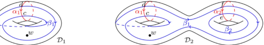
The Morse function fM and such a metric induce a Heegaard diagram for M, where the upper streamline γ(c) can be chosen as the termination of the actual streamline through c for the gradient current fM. Choose an external point w of the diagram and let γ(w) be the closure of the flow line through w with respect to g.

Parallels of flow lines

The cycle L(m) depends neither on the orientations of αi and βj nor on their order. Permuting the roles of αi and the roles of βj reverses its orientation, leaving lk(L(m), L(m)k) unchanged.

Since the change in orientation αi(c) leaves Jj(d)i(c)σ(c) invariant and the change in orientation βj(c) leaves Jj(c)i(d)σ(c) invariant, the cycle G (D) is not depending on the orientations αi and βj. It is also easy to see that permuting the roles of αi and βj reverses the orientations of γ(c), turns J into a transposed matrix, and does not change even the cycle of G(D).

In particular, our choices for a±i near ai (resp. for b±j ) do not matter as long as they satisfy our assumptions of being on the desired side of D(αi) (resp. now that + and - play the same roles in the formula, γ(c)k does not depend on the orientations of αi and βj.

Combinatorial definition of e(w, m)

Statement of the main theorem

A systematic study of variations of the three components of the formula under moves connecting two Heegaard diagrams of a rational 3-sphere homology is carried out in [Les14]. In this section, we introduce a propagator P(f,g) associated with a Morse function f without minima and maxima of ˇM, and with a metric g that is standard outside BM. Similar propagators associated with more general Morse functions have been constructed by Watanabe in [Wat12], independently.

Our standard representation of the horsehair Hb of [4,+∞[ under f in CM is shown in the upper part of figure 7. The two-dimensional increasing manifold of ai is oriented arbitrarily, its closure is denoted by Ai. The descending polynomial ai consists of two half-lines L+(ai) and L−(ai), which start as verticals and end at ai.

Symmetrically, the descending two-dimensional manifold of bj is arbitrarily oriented, its closure is denoted by Bj. The ascending manifold ofbj consists of two half-lines L+(bj) and L−(bj) that start atbj and end as vertical lines.

The propagator P (f, g)

For simplicity, UMˇ|γ(c) will sometimes be simply denoted by S2×γ(c), or by S2×τ γ(c) when the parallelization τ that induces such a diffeomorphism matters. Let's look at the part coming fromai, where the closures L+(ai) and L−(ai) of streamlines stop and closures of streamlines from Ai start. The two boundary parts (−L(ai))× Ai and Bj×(−L(bj)) intersect along a two-dimensional locus, and the 3-cycle ∂Pφ.

Proof: The interior of a figure similar to Figure 9 is embedded in the closure Ai of the increasing manifold of ai in ˇM. The full closure is obtained by attaching such an open disc to the ascending manifolds (L(bj) = L+(bj)− L−(bj)) of bj. Near the diagonal of such a line, Bj×Ai is parameterized by the height of the first point in [1,5] followed by the infinite difference (second point minus first point) parameterized by (height difference, αi,− ( −βj)), where a minus sign precedes βj.

Using the propagator to prove Proposition 3.4

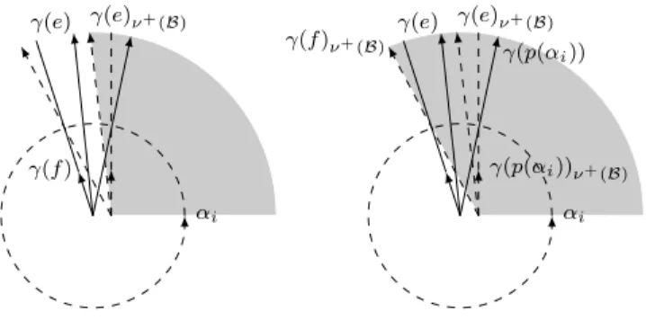
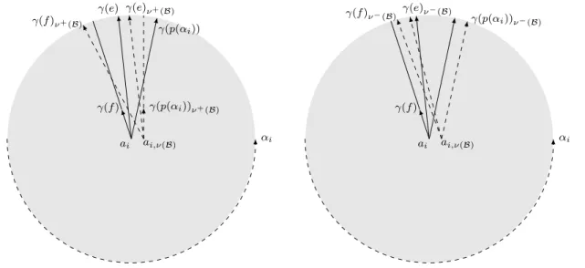
Recall from Lemma 4.1 that αi is the positive normal to Bj along streamlines through positive intersections. In particular, the orthogonal projections on Bj(d) of b+j(d) and b−j(d) both coincide with the intersection of the dotted segments in Figure 11, and the orthogonal projections on Ai(d) of a+ i( d) and a−i(d) both coincide with the intersection of the dashed segments in Figure 10 on a larger scale. Since the γ(c)ν(B) then crosses the Bj like the αi which are positive normals to Bj along streamlines associated with positive crossings.

The only difference comes from the fact that the streamlines are oriented toward bj(d) so that they cross Ai as (−βj) which is the positive normal along the streamlines associated with the negative transitions. Since the first ˇM-coordinate of a point in γ(c)ν(B)×γ(d)k is very close to γ(c), γ(c)ν(B)×γ(d)k expects Pφ in a neighborhood small ofai× He. The only points of intersection of γ(d)k with the domain D(γ(c)) of Ai are near bj and they are shown in figure 11.

Choose a natural trivialization (X1, X2, X3) of TMˇ on a regular neighborhood N(γi) of γi, such that:. the other streamlines never have X1 as an oriented tangent vector. X1, X2) are tangent to Ai (except for the parts of Ai near bi coming from other intersections of αi ∩βi), and (X1, X3) are tangent to Bi (except for the parts of Bi near ai that come. Note that X is tangent to Ai on N(γi) (except on the parts of Ai near bi which come from other intersections of αi ∩βi), and that X is tangent to Bi on N(γi) (except on the parts of Bi near ai) coming from other intersections of αi∩βi In Figure 14 (and in Figure 7), γi is a vertical segment, all other streamlines corresponding to intersections involving αi go upward fromai, and X is simply the upward vertical field.

The propagator associated with a combed Heegaard splitting

Introduction to specific chains P X and P −X

Y is tangent to the line L(bj) at bj, for any j, (again, Y need not direct the line).

Assume without loss that the isotope ψY moves the critical points rai along the lines L(ai) and bj along L(bj) (remember that Y is tangent to these lines). Furthermore, the direction of ​​ψ∗(φ) at the critical points and the direction of ​​φ at their images under ψ coincide with sa(−Y). Proof: The direction of ​​ψ∗(φ) along γ(c) is very close to the tangent direction of ​​γ(c) away from the ends of γ(c), and it deviates slightly in the orthogonal direction of sa(−Y ) ) since γ(c) is obtained from ψ(γ(c)) by a translation of −Y.

Near the critical points, the direction of ψ∗(φ) approaches the direction of sa(−Y) and reaches it at the critical points. Similarly, the direction of φ along ψ(γ(c)) is very close to the direction of (−T(γ(c))) away from the edges and is slightly deviated in the orthogonal direction of (−sa(Y )). In addition to those points, we need to look for streamlines for φ and streamlines for ψ∗(φ) that intersect twice and connect the intersection points with opposite directions.

Reduction of the proof of Proposition 6.1

Proof of Proposition 6.4

In particular, Gi↑↓(Y) can be thought of as the intersection of P(f,g)∩ P(−f,g) inside C2(M), while Gb↑↓(Y) collects the intersection coming from the boundary correction. Since ψ∗(φ) is nearly vertical away from the critical points, we are left with the behavior near the critical points. Near ai on Ai (or near bj on Bj) the direction ψ∗(φ) in the hemisphere is sa(−Y), according to Lemma 6.2, so that pairs of points Ai× Bj are connected by streamlines ψ ∗(φ) in near the critical point.

According to Lemma 6.2, the direction φonψ(Ai) is close to ψ(ai) (or onψ(Bj) is close to ψ(bj)) in the hemisphere sa(−Y), so that the pairs of points (ψ(Bj)×ψ (Ai ))∩ι(Pφ) near the critical points are again in N.

Proof of Proposition 6.5

This can only happen in the tubular surroundings γi at the point where the streamlines ψ∗(φ) and φ have the same horizontal direction. This happens only between γi and ψ(γi), more precisely in the rectangle shown in Figure 17 under the rectangular projection directed by X1. Indeed, since the horizontal component of the direction ψ∗(φ) along γ(c) is in the sa(−Y) direction, Ψ(Ph)∩(S2×L) =O(N). Now (− X) can belong to [ψ∗(φ), ψ∗(X)] if the direction of the horizontal component of (−X), which is the direction of the horizontal component of sφ, is the same as the direction of the horizontal component of sψ ∗(φ ).

This can only happen in the same rectangles as before, where (−X) is in the hemisphere of sa(−Y). Note that X depends neither on the orientations of αi and βj nor on their order. Therefore, thanks to Proposition 6.1, the proof of Theorem 3.8 is reduced to the proof of the following equality iH2(UMˇ;Q).

Proof: If Y extends as a non-zero part of X⊥(Σ) still denoted Y, then the cycle of the left side bounds s[−X,X]Y(Σ). The proof of Theorem 3.8 has now been reduced to the proof of the following theorem, which appears at the end of this section. The theorem thus implies that the sum e(w,m) is independent of our special view of the Heegaard diagram.

A surface Σ(L(m))

Computehαk, ui, by pushing in the direction of the positive normal to αkand in the direction of the negative normal and by averaging, so that locally.

Proof of the combinatorial formula for the Euler classes

Similarly, assume that the curves α are orthogonal to the figure in the lower parts of the handles in the standard figure of Hbin Figure 7, and draw a planar view similar to Figure 19 of Ha,4m (which is f−1(4) ∩CM minus the disc neighborhoods of preferred transitions), starting with Figure 21 and adding a vertical band cut by a horizontal arc of βj oriented from right to left, for each βj. Expand each Y =Yε,η in Hb so that Y appears constant and horizontal in our standard figure of Hb in Figure 7 and so that its projection in Figure 21 is the constant drawn field. Also suppose that each Y = Yε,η varies in a quarter of the horizontal plane in our tubular neighborhoods of theγi in Figure 14 .

Proof: Take the arc [c, d]β between two consecutive intersections β. The η-normal is a positive normal when η = + and a negative normal otherwise). This (−η)-normal starts and ends vertically in this figure, and Yε,η is horizontal with a direction that depends on the sign of ε. Therefore, the sum of the degrees (−η) of the normal in the direction Yε,η and in the direction Y(−ε),η is 2de(|c, d|β).

Lescop - "Sur la construction de Kontsevich-Kuperberg-Thurston d'un invariant d'espace de configuration pour l'homologie rationnelle 3-sphères", math.GT. Marin - "Un nouvel invariant pour les sphères d'homologie tridimensionnelle (d'après Casson)", Ast'erisque (1988), no.