HAL Id: hal-00857362
https://hal.archives-ouvertes.fr/hal-00857362
Submitted on 3 Sep 2013
HAL is a multi-disciplinary open access archive for the deposit and dissemination of sci- entific research documents, whether they are pub- lished or not. The documents may come from
L’archive ouverte pluridisciplinaire HAL, est destinée au dépôt et à la diffusion de documents scientifiques de niveau recherche, publiés ou non, émanant des établissements d’enseignement et de
To cite this version:
Serge Guillaume, Brigitte Charnomordic, Patrice Loisel. Fuzzy partitions: a way to integrate expert knowledge into distance calculations. Information Sciences, Elsevier, 2013, 245, p. 76 - p. 95.
�10.1016/j.ins.2012.07.045�. �hal-00857362�
Fuzzy partitions: a way to integrate expert knowledge into distance calculations
Serge Guillaumea, Brigitte Charnomordicb, Patrice Loiselb
aIrstea, UMR ITAP, BP 5095, 34196 Montpellier, France
bINRA-SupAgro, UMR 729 MISTEA, F-34060 Montpellier, France
Abstract
This work proposes a new pseudo-metric based on fuzzy partitions (FPs).
This pseudo-metric allows for the introduction of expert knowledge into dis- tance computations performed on numerical data and can be used in various types of statistical clustering or other applications. The knowledge is formal- ized by a FP, in which each fuzzy set represents a linguistic concept. The pseudo-metric is designed to respect the FP semantics. The univariate case is first studied, and the pseudo-metric behavior is discussed using synthetic experiments. Then, a multivariate version is proposed as a Minkowski-like combination of univariate distances or semi-distances. The value of the pro- posal is illustrated with two real-world case studies in the fields of Biology and Precision Agriculture.
Keywords: semi-supervised, metric, expert knowledge, clustering, segmentation
1. Introduction
Clustering procedures are common statistical data analysis techniques used in many fields. Clustering can be of various types, mainly hierarchical algorithms and partitional algorithms. Different types of data are candidates for clustering, including numerical data, categorical data and more complex types of data, such as graphs and multimedia data. The clustering of nu- merical data is frequently addressed in the literature, with well-established methods such as k-means for partitioning. However, these methods do not
Email address: serge.guillaume@irstea.fr(Serge Guillaume)
allow for the incorporation of expert knowledge. Although challenging, the use of conjointly numerical data and expert knowledge may be a good way to guide clustering procedures using a semi-supervised approach and to improve clustering results.
Zadeh proposed the concept of the linguistic variable [30] to implement approximate concepts and reasoning. The goal was to ease the contribution of domain experts to system modeling. A fuzzy set, defined by its membership function, determines a symbol, called a linguistic concept, in the numerical space. The FP is then composed of the fuzzy sets corresponding to each of the linguistic labels. Other approaches, based on ontologies, can be used to formalize domain knowledge, as described, for instance, in [20]. However, these approaches essentially use symbolic information, and the numerical aspects are difficult to introduce.
The fuzzy set representation framework combines numerical and symbolic aspects and cannot be reduced to either of these paradigms.
Our objective in this paper is to take advantage of the linguistic variable concepts to use numerical and symbolic information related to the same variable together in the same clustering procedures, which is not typical in clustering. Clustering methods are designed to address several types of variables, e.g., numerical or symbolic variables, without combining different types of information for a given variable.
Most clustering or classification techniques are based on a function d, which determines how the dissimilarity of two elements is calculated, as follows: between individuals, between individual and group or between groups.
Clustering results are sensitive to the choice of the dissimilarity function [1, 14].
The combination of numerical and symbolic information and its introduc- tion into the dissimilarity function would allow for its use in any clustering method or, more generally, in any dissimilarity-dependent algorithm.
The dissimilarity function must have the properties of non-negativity and symmetry and satisfy the triangle inequality, and it can be proper (identity of indiscernibles) or semi-proper. In the first case, the dissimilarity function is a metric or distance. In the second case, the dissimilarity function is a pseudo-metric or semi-distance.
The most common metrics for numerical values are defined by the Lp norms:
kxkp = (|x1|p+. . .+|xn|p)p1
where xis a multidimensional vector (x1, x2. . . xn). The classical case of the Euclidean norm is obtained for p= 2.
Other distances can be used in multivariate problems in which variables are not independent, for instance, the Mahalanobis distance or the Cho- quetMahalanobis operator [26].
Dissimilarity functions have also been defined for non-ordered categorical data, e.g., material={plastic, metal, wood}. The definition of a dissimilarity function is mainly based on the presence or absence of a given attribute. In [3], several similarity measures are compared. Some of these similarity mea- sures consider the sample size, the number of values taken by the attribute and the frequencies of these values in the data set. The Lorentz curve allows for the ranking of multi-attribute categorical data [9]. To our knowledge, scant attention has been paid to similarity measures for ordered categorical data, such as price={cheap, average, expensive}. In this case, the distance betweencheapandexpensivemust be higher than the distance betweencheap and average and the distance between average and expensive. Ordered cat- egorical data can be represented by linguistic variables, based on fuzzy sets, with each concept corresponding to a given fuzzy set.
Like many other concepts, the concept of distance has been generalized to fuzzy sets. In a survey [2], Bloch recalls the three types of fuzzy distances already defined: between two points in a fuzzy set, from a point to a fuzzy set and between two fuzzy sets. Many studies tackle this problem, including [8, 6, 19, 10, 5]. Certain proposals pay attention to the fulfillment of the triangle inequality [4]. Recent developments consider distance and similarity measures suited for new types of fuzzy sets, including interval-valued [31], intuitionistic [28] or hesitant [29] fuzzy sets, or try to define a new family of metrics for compact and convex fuzzy sets [27], which is useful for imprecise data analysis. Distances in rough set theory [18] and evidence theory [16]
have also recently been analyzed in surveys.
Bloch [2] does not mention the distance between individuals within a FP. Such a distance has been little studied. Based on the membership de- grees, such a distance would be valid for numerical measurements while also containing a symbolic component related to the granularity of information.
A FP carries semantics and knowledge about variable behavior. For the semantics attached to the partition-related concepts to be valid, the distance between two non-distinguishable elements must be equal to zero, which is the case for all of the elements within a given fuzzy set kernel. Furthermore, elements belonging to different concepts must always have a distance higher
than elements belonging to the same concept.
In [11], a first attempt at designing this type of distance has been proposed to build a hierarchy of FPs. The initial partition was defined as a strong fuzzy partition (SFP) with as many fuzzy sets as distinct values for the given variable. Then, at each step, two adjacent fuzzy sets were merged into one new fuzzy set. The selected pair was the pair that yielded the minimum variation in the sum of distances for the entire training set. The objective of this process was to preserve the structure of the previous step.
The objective of the present work is different. The distance is not used to build a FP, but the FP is used to introduce expert knowledge into distance calculations.
Beginning with the preliminary study presented in [13], this paper pro- poses to take advantage of fuzzy set formalism to add a semi-supervised aspect to distance-based statistical procedures such as clustering. The semi- supervision is performed by using available expert knowledge to superimpose linguistic concepts onto numerical data. This pretreatment is followed by the design of a pseudo-metric based on the FPs corresponding to the concepts and its use in clustering procedures. The procedure is thus an approach to combine numerical data and imperfect data resulting from human judgment.
The paper is organized as follows. Section 2 introduces a function based on FPs to calculate the dissimilarities between univariate points. Various areas are considered in the FP, and the function is designed accordingly to constitute a system of embedded functions. Then, the pseudo-metric prop- erties are demonstrated. Section 3 discusses the particular case of SFPs.
Section 4 studies the pseudo-metric behavior in depth and includes a com- parison with the Euclidean distance, synthetic experiments and a real-world case study. A multivariate pseudo-metric is proposed in Section 5 that illus- trates a real-world case study using partitioning methods. Section 6 provides conclusions.
2. The proposed function and its properties
The proposal applies to data in the unit interval U = [0,1] and relies on FPs.
2.1. Notations and constraints on the fuzzy partition
Denote byP the FP composed off fuzzy sets, defined by their respective membership functions (MFs) labeled 1,2. . . f.
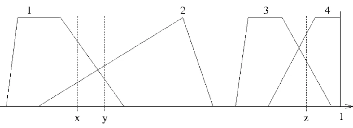
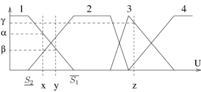
Figure 1: Example of FP and data points x,y,z
Denote byd∗(x, y) the proposed function for FP P. Denote byµi(x) the membership degree of x in the MF i.
Denote bySi = [Si, Si] the support of MF i, defined by{x|µi(x)>0}. Denote byKi = [Ki, Ki] the kernel of MF i, defined by{x|µi(x) = 1}. By convention, K0 = K0 = S0 = 0, Kf+1 = Kf+1 = Sf+1 = 1 and
∀x∈U, µ0(x) = µf+1(x) = 0.
The FP must respect the following constraints:
• it is composed of linear triangle or trapezoid MFs,
• any point belongs to two MFs at most, and
• ∀i∈[1, f],∃ x such as µi(x)>0 andµj(x) = 0, ∀j 6=i.
Rationale: The whole set of constraints is related to the MF distinguisha- bility considerations, which is necessary for semantic reasons because the MFs represent linguistic concepts.
The linear triangle or trapezoid MFs are chosen for the sake of simplicity and because they have a bounded support. The limitation for any point to have at most non-null memberships in 2 MFs corresponds to the semantics of the FP. Each MF represents a concept, which is part of an ordered sequence.
Therefore, any point should be either a prototype of a concept or a transition between two concepts. The last constraint requires that the kernel have at least one exclusive prototype, which prevents the support of a given MF from going beyond the kernel of the following MFs.
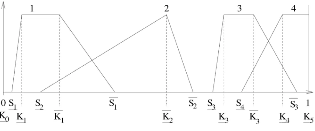
An example of a partition satisfying the constraints is shown in Figure 1, and the notations are illustrated in Figure 2.
Figure 2: Notations for a FP
2.2. Desirable behavior
The proposed FP-based function combines numerical and symbolic el- ements. The numerical elements allow for the function to handle multiple memberships in transition zones, whereas the symbolic elements consider the granularity of the concepts associated with the fuzzy sets.
To ensure a smooth transition between concepts and a smooth behavior within a given MF, the proposed function d∗(x, y) must be continuous and non-decreasing when x and y move away from each other. The MFs must provide a structure to the distance calculation so that all points within a kernel have a null distance and so that d∗(x, y) = |j−i| forx∈Ki, y ∈Kj. Semi-distance properties, which will be detailed in Section 2.5, are re- quired for the proposed function. Thus, the function can be introduced into a wide range of applications including clustering and segmentation.
Many possible combinations of numerical and symbolic elements may be studied, but it is difficult to design a function that behaves like a semi- distance. To explain our choice, we first study the case of data pairs lying within overlapping MF areas and then provide the general formula for the proposed function.
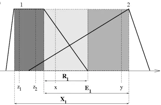
Figure 3: Various types of overlapping areas Restricted (R
1), Embedded (E
1), eXtended (X
1)
2.3. Decomposition into areas
We define three types of overlapping areas, examples of which are shown in Figure 3:
Definition 2.1. (i) Let Xi = [Ki, Ki+1[, for 0 ≤i ≤ f, the eXtended over- lapping area.
(ii) Let Ei ⊂Xi, the Embedded overlapping area: Ei = [Ki, Ki+1[.
(iii) Let Ri ⊂Ei, the Restricted overlapping area, defined by:
Ri =cl{x∈Ei|µi(x)>0, µi+1(x)>0} where cl is the closure operator.
To summarize, we have Ri ⊂Ei ⊂Xi and Xi =Ei∪Ki,∀i∈[1, f].
In the example given in Figure 3, we have R1 = [K1, S1], but this is not always true, depending on the support and kernel locations.
For each overlapping area and the total area, we propose distinct func- tions that, as we will demonstrate in Section 2.6, constitute a system of embedded pseudo-metrics.
2.3.1. Within restricted overlapping areas
To obtain a smooth behavior, the function is reduced to a numerical component dn that is based on the four membership degrees in the two MFs present within the restricted area:
Definition 2.2. Letx, y ∈[0,1]be any two points within the restricted over- lapping area Ri. The numerical component dn is given by:
∀x≤y ∈Ri, dn(x, y) =µi(x)µi+1(y)−µi+1(x)µi(y)
∀x > y ∈Ri, dn(x, y) =dn(y, x) (1) From Definition 2.2, we deduce the following property:
Proposition 2.1. The dn value satisfies dn(x, y)>0 if x6=y.
Proof: easily deduced from µi(x)> µi(y), µi+1(y)> µi+1(x).
2.3.2. Within embedded overlapping areas
The embedded overlapping area is composed of a core, defined previously as the restricted overlapping area, surrounded (or not) by two subareas in which only one MF is present. Because the number of non-null membership degrees to consider varies depending on the location of the fuzzy set bounds, it is easier to define the d0 function, which is valid within the embedded overlapping areas, as a sum of three terms, each of which corresponds to one of these subareas.
Definition 2.3. Letx, y ∈[0,1]be any two points within the embedded over- lapping area Ei. The numerical component d0 is given for all x≤y ∈Ei,:
d0(x, y) = 1 Ni
[µi(x)−µi(min(y,max(x, Si+1))) +dn(max(x, Si+1),min(y, Si))
+µi+1(y)−µi+1(max(x,min(y, Si)))]
(2)
with Ni = 1−µi(Si+1) +dn(Si+1, Si) + 1−µi+1(Si),1≤i≤f −1 N0 =Nf = 1
and for all x > y ∈Ei, d0(x, y) =d0(y, x).
Remarks:
1. Definition 2.2 is extended to data pointsx, y /∈Ri, so that, in this case, dn(x, y) = 0.
2. In Equation (2), min and max are introduced to comply with the va- rious possible locations of the data points within the Ri and Ei −Ri
subareas.
3. The normalization coefficientNiguarantees that∀x, y, d0(x, y)∈[0,1].
Example: Let us consider the values x, y shown in Figure 3. In this case, the first element of do(x, y) is equal to zero, the second element is equal to dn(x, S1) and the last element is equal to µ2(y)−µ2(S1).
2.3.3. Within extended overlapping areas
By convention, all points that belong to a given MF kernel, such as z1
and z2 in Figure 3, are considered to have a null distance. This convention is necessary to respect the fuzzy set semantics. Thus,
∀i∈[1, f],∀x, y ∈[Ki, Ki]⇒d∗(x, y) = 0
Therefore, d∗(Ki, Ki) = 0. Hence, in extended overlapping areas, we define the d1 function using the d0 function in embedded overlapping areas:
Definition 2.4. Letx, y ∈[0,1]any two points within the extended overlap- ping area Xi. The numerical component d1 is given by:
∀x, y ∈Xi, d1(x, y) = d0(max(x, Ki),max(y, Ki)) (3) 2.4. Proposed function in the whole domain
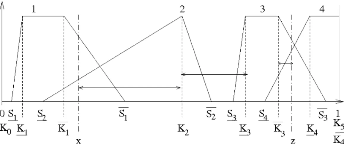
When the data points do not lie within the same overlapping area, as is the case for points x and z in Figure 4, the formula is more complex and contains a numerical componentd1, which reflects the relative location within the extended area to which each point belongs, and a symbolic component, which accounts for the number of MFs between the points.
Figure 4: FP-based univariate function calculation; arrows represent the partial distances to be combined
We denote by I(x) the function such that:
∀i∈[0, f], x∈Xi ⇔I(x) =i
The functiond2(x, z) is calculated as a sum of partial elements associated with various areas: the area from x to the kernel of the (I(x)+1)th MF, the
area between the kernels of the (I(x)+1)th and the I(z)th MF and the area from the kernel of the I(z)th MF to z.
Forsemanticconsiderations, the distance between the two kernels of MFs I(x) and I(z) is assumed to be the distance between the two corresponding linguistic concepts. It is a symbolic element, equal tods(I(x), I(z)) =|I(z)− I(x)|, which does not depend on the MF bounds. The following formula is proposed:
Definition 2.5. Let x, z ∈[0,1] be any two points. For all x≤z, d∗(x, z) =
(d1(x, z) if I(x) =I(z)
d1(x, KI(x)+1) +ds(I(x) + 1, I(z)) +d1(KI(z), z) if I(x)< I(z) (4) where ds(i, j) =|j −i|, ∀i, j ∈[1, f −1].
For all x > z, d∗(x, z) =d∗(z, x).
If f is large, the term using ds becomes predominant, while the terms involving d1 have a relatively limited influence, withd1 being between 0 and 1. This is expected to reflect the expert knowledge.
The various parts of the sum in Equation (4) are illustrated by the arrows in Figure 4. In this case, we have I(x) = 1 and I(z) = 3.
According to Equation (4), the symbolic component is zero when I(z) = I(x) + 1. In this case, xand z are located on both sides of a given fuzzy set kernel.
The d∗ distance could be used as such. The upper bound of the distance may take the following values, f − 1, f, f + 1, according to the partition edges. The dependence on f can be a problem if one wants to compare FPs of various sizes. To address this issue and achieve a better commensurability between the different terms, normalization is proposed. The general formula becomes
dP(x, y) = d∗(x, y)
f −1 +d0(0, K1) +d0(Kf,1) (5) where f is the number of fuzzy sets and P stands for a given FP. In the equation, d0(0, K1) andd0(Kf,1) may take 0 or 1 values.
This normalization may hide the level of granularity chosen by the ex- pert. If no comparison is required between FPs of various sizes, d∗ should be preferred.
The properties of dissimilarities, semi-distances and distances are now recalled before demonstrating which of the properties are satisfied by the proposed function dP.
2.5. Distance properties
A functiond is a dissimilarity if
∀x, y ∈U,
d(x, y)≥0 d(x, x) = 0 d(x, y) = d(y, x)
A dissimilarity is semi-proper if d(x, y) = 0 ⇒ ∀ w, d(x, w) = d(y, w), and it is proper if d(x, y) = 0⇒x=y.
A semi-distance is a dissimilarity that verifies the triangle inequality:
∀x, y, z ∈U, d(x, y)≤d(x, z) +d(z, y) (6) A proper semi-distance is called a distance. In this paper, the goal is not to ensure the proper character because all kernel elements must be indistin- guishable. The expected properties are those of a semi-distance.
2.6. Checking properties
Let us examine the cases that correspond to the different areas, where Equations (1), (2), (3), (4) or (5) are applicable.
1. Properties of the function dn on restricted overlapping areas Let us prove that dn is a distance.
Proposition 2.2. The function dn is a distance. It is symmetric by construction.
Proof: dn is obviously a dissimilarity. We have to prove that dn is proper and satisfies the triangle inequality.
(i)dn is proper: if we assumedn(x, y) = 0, thenµi(x)µi+1(y) = µi(y)µi+1(x).
As µi(x)≥µi(y) and µi+1(y)≥µi+1(x), we deduce thatµi(x) =µi(y) and µi+1(y) = µi+1(x). Therefore, x=y.
(ii) dn satisfies the triangle inequality:
Leta =Si+1 andb=Si. Because the MFs are linear functions,µi(x) = si(b−x), wheresi is a positive coefficient. Similarly,µi+1(x) =si+1(x− a), where si+1 >0. We consider three cases:
(iia) z < x < y. It is sufficient to show that dn(x, y)≤dn(z, y):
dn(z, y)−dn(x, y) = (µi(z)−µi(x))µi+1(y)−µi(y)(µi+1(z)−µi+1(x))
=sisi+1[(x−z)(y−a)−(z−x)(b−y)]
=sisi+1(x−z)(b−a)≥0
(iib) x < z < y. The inequality (6) to be verified becomes
∀x, y, z ∈Ri, µi(x)µi+1(y)−µi(y)µi+1(x)≤µi(x)µi+1(z)−µi(z)µi+1(x) +µi(z)µi+1(y)−µi(y)µi+1(z) which can be rewritten as
(µi(y)−µi(z))(µi+1(y)−µi+1(x))≤(µi(x)−µi(y))(µi+1(z)−µi+1(y)) Therefore, using µi, the previous inequality becomes
(z−y)(y−x)≤(y−x)(z−y).
Thus, the triangle inequality is proven.
(iic) x < y < z, which has the same proof as that for case a.
2. Properties of thed0 function on embedded overlapping areas.
The definition of d0 is based on the addition of the Euclidean distance and the distance dn on disjoint intervals. Therefore, d0 is a distance.
3. Properties of thed1 function on extended overlapping areas
In the case of kernels reduced to a single point, the definition of d1
reduces to the distance d0. Therefore, d1 is a distance. Otherwise, d1
is not proper but is only semi-proper. Therefore, in general, d1 is a semi-distance.
4. Properties of thed∗ function (and then dP)
The definition of d∗ is based on the addition of the numerical semi -distance d1 and the symbolic distanceds on disjoint intervals. There- fore, d∗ (and thereforedp) is a semi-distance.
3. The particular case of strong fuzzy partitions
A SFP, described by f membership functions on the universe U, fulfills the following condition:
∀x∈U,
f
X
i=1
µi(x) = 1 (7)
Figure 5: Example of a SFP
An example of SFP is shown in Figure 5.
Because of the SFP structure, the following relationship always holds:
∀i∈[1, f−1], ∀x∈U, µi(x) +µi+1(x) = 1 Equation (1) becomes:
dn(x, y) = µi(x)−µi(y)
Thus, for SFPs, the numerical component is defined only by the mem- bership degrees to a single MF, the first MF in the partition order. For the example shown in Figure 5, dn(x, y) = α−β.
Within the restricted overlapping area,
∀x∈Ri, µi(x) = 1− x−Si+1
Si−Si+1
Thus, given two points inRi,dn(x, y) = |y−x| Si−Si+1
is directly proportional to the Euclidean distance between the two points.
Because of the SFP structure, Ri ≡ Ei, and the corresponding function satisfies d0 ≡dn.
After further simplification, Equation (4) becomes
∀x, y ∈U, d∗(x, y) =|µI(x)(x)−µI(y)(y) +I(y)−I(x)|
The P-based univariate pseudo metric is:
∀x, y ∈U, dP(x, y) = |µI(x)(x)−µI(y)(y) +I(y)−I(x)|
f −1 (8)
Equivalent definition from a function
The SFP-based proposed pseudo-metric can also be designed using a func- tion.
Let us introduce the function P:
P(x) = I(x)−µI(x)(x) (9)
P is a positive non-decreasing function of x and is increasing in overlapping zones.
dP(x, y) can then be written as
dP(x, y) = |P(y)−P(x)|
f −1 (10)
This formulation, which shows that the use of SFPs is an elegant alternative to data transformation, also makes it easier to check the properties of SFP- based pseudo-metrics.
The quality of SFPs has been previously highlighted in the past. Pedrycz [22] noted that SFPs are error-free reconstructions for Sugeno-type systems using centroid defuzzification:
∀x∈U, ψ[φ(x)] =x
where φ is the input space transform and ψ is the output space transform.
Euclidean distance and regular fuzzy partitions
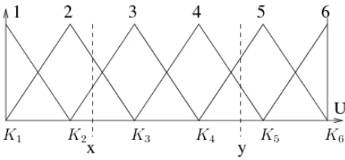
Definition 3.1. A regular fuzzy partition is composed of triangular MFs, with equidistributed kernel centers K1. . . Kf, with Ki =Si−1 =Si+1.
A regular fuzzy partition with six MFs is shown in Figure 6.
Figure 6: A regular fuzzy partition
For this particular case, we show that the proposed pseudo-metric is a metric and that it yields the same result as the Euclidean distance, regardless of the number of terms in the partition.
The regular distribution of the fuzzy set centers allows for the simplifica- tion of Equation (3) because data are normalized in the unit interval:
K1 =S1 = 0 and∀i >1, Ki =Si+1 =Si = i−1 f −1 which yields Si−Si+1 = 1
f −1.
The function P, defined in Equation (9), becomes P(x) = (f −1)x, and finally, d(x, y) =|y−x|.
The Euclidean distance and the regular SFP-based metric are identical when the data are in the unit interval.
This equivalence results because the distance proposed in Equation (5) distorts the Euclidean distance according to the two following points: the symbolic distance between concepts and the indistinguishability of the kernel elements. In the case of a regular SFP, these two characteristics disappear because all kernels are reduced to single points and are equidistant.
4. Behavior and illustration in the univariate case
This section investigates the univariate pseudo-metric behavior and illus- trates its utility. This section compares the univariate pseudo-metric with the Euclidean distance and provides two examples of use of the univariate
pseudo-metric: synthetic experiments using hierarchical clustering and a real- world case study with a segmentation algorithm.
4.1. Comparison with the Euclidean distance
Let us highlight two important properties of the proposed FP-based pseudo-metric.
First, the FP-based pseudo-metric value is always zero for any two points that belong to the same fuzzy set kernel.
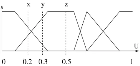
Second, the dP pseudo-metric is typically different from the Euclidean distance, and the deviations depend on the fuzzy set slope and kernel width.
These deviations may produce a different ranking compared with the Eu- clidean distance, as shown in Figure 7. The three points x, y, z have co- ordinates 0.2, 0.3, 0.5. According to the Euclidean distance, denoted by dE,
dE(x, y) = 0.1 < dE(y, z) = 0.2 and when the F P-based pseudo-metric is used,
dP(y, z) = 0.067 < dP(x, y) = 0.133
0 1
x y z
0.2 0.3 0.5
U
Figure 7: An example of an inversion compared to the Euclidean distance
4.2. General behavior
The proposed pseudo-metric behavior is likely to depend on two main characteristics of the FP: the number of linguistic concepts, which affects the symbolic component, and the size of the different kernels, with the wider the kernels having more numerous indistinguishable values.
It would be difficult to conduct a separate study of the influence of the various parameters because the parameters influence one another. Therefore,
Algorithm 1: The partition generation algorithm
1 Input Number of MFs, NM F; Cumulative kernel size, K
2 Output FP kernel bounds, Kbounds 3 Initialize cumulative kernel size: k = 0.
4 Random setting of NM F −2 centers.
c={c1 = 0, c2, . . . , cNM F−1, cNM F = 1}
5 The centers are used to initialize kernel bounds.
Kbounds ={c1, c1, . . . , cNM F, cNM F}
6 while k ≤K do
7 m=Random[1, NM F] // Select MF to be modified
8 s=Random[0,1]// Generate a new kernel size
9 if ((k+s ≤K) & (MFs still distinguishable)) then
10 Kbounds[m] ={cm−s/2, cm+s/2}
11 k =k+s
12 end
13 end
14 a=K−k // Update the last MF kernel size
15 Kbounds[m] ={cm+a/2, cm−a/2}
numerical simulations have been undertaken to investigate the general behav- ior of the distance. Various SFPs have been randomly generated according to Algorithm 1.
The two input parameters of the generation algorithm areNM F(>2), the number of MFs, andK, the cumulative kernel width over the partition. The first and last MF centers are set to 0 and 1 to address the case in which the cumulative size of kernels is zero, i.e., when all MFs are triangular in shape.
The distinguishability constraints mentioned in Algorithm 1 are such that when an MF is modified, its new lower (upper) kernel bound is still higher (lower) than the upper (lower) kernel bound of the previous MF.
The partitions are characterized using a regularity index, defined as follows:
Definition 4.1. LetP be any partition composed ofNM F trapezoidal or tri- angular MFs over the same definition domain D. The ith MF kernel of P is denoted by [Ki, Ki].
The regularity index of P is defined by comparison with a regular fuzzy partition RP of size NM F (see Definition 3.1). The ith MF kernel of RP is denoted by ci.
RI(P) = 1
√NM F −2
NM F
X
i=1
di(ci, P), with di(c, P) =
0, if c ∈[Ki, Ki]
min(dE(c, Ki), dE(c, Ki)), otherwise
(11)
The FP is designed to distort the Euclidean distance. To evaluate the impact of a given partition on this distortion, N points are equally spaced in the unit interval, and the following distortion estimation is computed over all pairs of points.
DDE(P) = 1
q1
2(N2−N) v u u t
N
X
j=1 N
X
k=j+1
(dE(xj, xk)−dP(xj, xk))2 (12)
The random partition generation is performed according to Algorithm 1 for all combinations ofNM F from 4 to 10 andK ∈ {0,0.05,0.1,0.15,0.2,0.25,0.3}; the number of points N is set to 100, and the entire procedure is repeated 100 times. Numerical experiments showed thatRI(P) has a similar expectation, independent of the value of NM F, calculated over the sample experiments
●
●
●
●
●
●
●
●
●
●
●
●
● ●
●
●
●
●
●
●
●
●
●
●
●
●
●
●
●
●●
●
●
●
●
●
●●
●
●
●
●
●
●
●
●
●
●
●
●
●
●
●
●
●
●
●
●
●
●
●
●
●
● ●
●
●●
●
●
●
●
●
●
●
●
●
●
●
●
●
●
●
●
●
●
●
●
●
●
●
●
●
●
●
●
●
●
●
●
0.0 0.2 0.4 0.6 0.8 1.0
0.000.050.100.150.200.250.30
Partition regularity index
Distance distortion estimation ●
●
●
●
●
●
●
●
●
●
●
●
●
● ● ●
●
● ●
●
● ●
●
●
●●
●
●
●
●
●
●
●
●
●
●
●
●
●
●
●
●
●
●
●
●
●
●
●
●
●
●
●
●
●
●
●
●
● ●
●
●
●
●
●
●
●● ●
●
●
● ●
● ●
●
●
●
●
●
●
●●
●
●
●
●
●
●
●
●
●
●
●
●
●
● ●
●
●
●
●
●
●●
●
●
●
●
●
●
●
●
●
● ●
●
●
●
●● ●
●
●
●
●
●
●
●●
●
●
●
●
●
●
● ●
●
●
●
●
●
●
●
●
●
●
●
●
●
●
●
●
●
●
●
●
●
●
●
●
●
●
●
●
●
●
●
●
●
●
●
●
●
●
●
●
● ●
●
●
●
●●●
●
●
●
● ●
●
●
●
●
●
●
●
●
●
●
●
● ●
●
● ● ●
●
●
●
●
●
●
●
●
●●
●
●
●
●
●
●
●
●
●
●
●
●
●
●
●
●
● ●
●
●
●
●
●
●
●
●
●
●
●
●
●
●
●
●
●
●
●
●
●
●
●
●
●
●
●
●●
●
●
●
●
●
●
●
●●
●
●
●
●
●
●
●
●
●
●
●
●
●
●● ●
●
●
●
●
● ●
●
●
●
● ●
●
●
●
●● ● ●
●●
●
●
●
●
●
●
●
●
●
●
●
●
●
●
●
●
●
●
●
●
● ●
● ●
●
●
●
●●
●
●●
●
● ●
●
●
●
● ●
● ●
●
●
● ●
●
●
●
● ●
●
●
●
● ●
●
●
●
●
●
●●
●
●
●
●
●
●
●
●
● ●
●
●
●
●
●●
●
●
●
● ●
●
●
●
● ●
●
●
● ●
●
● ●
●
●●
●
●
● ●
●
●
●
●
●●
●
●
●
●
●
●
●
●
●
●
●
●
●
●●
●
●
●
●
●
●
●
●
●
●
●
●
●
●
●
●
●
●
●●
●
●
●
●●
●
●
●
●
●
●
●
●
●
●
●
●
●
●
●
●
●
●
●
●
●
●
●
●
●
●
●
●
●
●
●
●
●
●
●
●
●
●
●
●
●
● 4 MFs 5 MFs 6 MFs 7 MFs 8 MFs 9 MFs 10 MFs
● 4 MFs 5 MFs 6 MFs 7 MFs 8 MFs 9 MFs 10 MFs
● 4 MFs 5 MFs 6 MFs 7 MFs 8 MFs 9 MFs 10 MFs
● 4 MFs 5 MFs 6 MFs 7 MFs 8 MFs 9 MFs 10 MFs
● 4 MFs 5 MFs 6 MFs 7 MFs 8 MFs 9 MFs 10 MFs
● 4 MFs 5 MFs 6 MFs 7 MFs 8 MFs 9 MFs 10 MFs
● 4 MFs 5 MFs 6 MFs 7 MFs 8 MFs 9 MFs 10 MFs
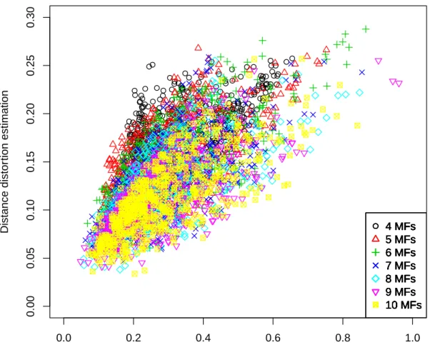
Figure 8: Illustration of the general behavior
(0.268 < E[RI(P)] < 0.297 for NM F between 5 to 10). This justifies the chosen normalization in Equation (11).
Figure 8 shows the results of the 100 experiments for each of the config- urations, with the regularity index RI(P) as the abscissa and the distance distortion estimation DDE(P) as the ordinate. The color and shape of the points correspond to a given number of MFs, regardless of the cumulative size of the kernels.
The linear regressions ofDDE versusRI, calculated independently for a given number of MFs, yield similar results: the slope, which varies between 0.202 and 0.238 forNM F between 5 and 10, and theR2 coefficient are similar.
The model that predicts the distance distortion according to the partition regularity index explains half of the variance (R2 ≈0.5, forNM F between 5 and 10), meaning that because of proper normalization, the distance behavior is not significantly influenced by the number of MFs in the partition. Instead, the distance behavior is influenced mostly by its regularity. The proposed index is one way to estimate this regularity and could certainly be improved.
The case of NM F = 4 differs slightly, with a lower slope of 0.155, a greater expectation (0.332) and a smaller R2 = 0.279.
These numerical experiments illustrate a general trend because the par- titions are randomly generated with little constraint and therefore vary sig- nificantly. The next section highlights the influence of the kernel size for partitions in which the deformation is more limited.
4.3. Synthetic case study
We will now examine the pseudo-metric behavior using a synthetic case study with univariate hierarchical clustering. Abottom up approach is used:
each observation begins in its own cluster, and pairs of clusters are merged as we move up the hierarchy. At each step, the selected pair of clusters to be merged is the pair that yields the minimum increase of within-group variance. The dendrogram can be analyzed to determine the composition of the clusters at a given hierarchical level.
The considered synthetic variable is wind speed. The speed, measured in either mph or km/h, is usually expressed through a partition endowed with natural semantics: the Beaufort scale1. Thirteen degrees are defined in the range of [0−120] km/h. Higher degrees have wider ranges of speed.
1http://en.wikipedia.org/wiki/Beaufort scale
For example, the range of degree 2, labeled Light Breeze, is [5.6−11] km/h, whereas the range of degree 5, Fresh Breeze, is [29−38] km/h.
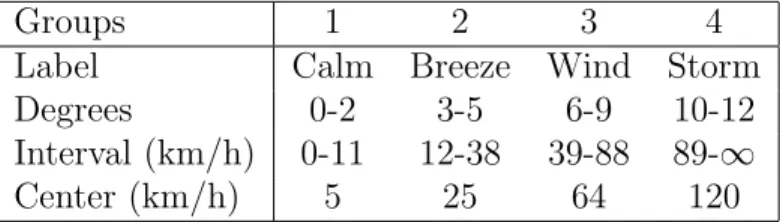
To simplify the study, the degrees are placed in four groups, each of which consists of approximately three degrees. The group characteristics are summarized in Table 1.
Table 1: The four groups of Beaufort degrees
Groups 1 2 3 4
Label Calm Breeze Wind Storm
Degrees 0-2 3-5 6-9 10-12
Interval (km/h) 0-11 12-38 39-88 89-∞
Center (km/h) 5 25 64 120
The impact of the pseudo-metric behavior on the hierarchical clustering procedure, implemented ashclustin theRenvironment[23], is analyzed. The results are highly sensitive to two factors: the choice of the metric between individuals and the method chosen for agglomerating the clusters. In the present study, the centroid agglomeration method is used as the method for agglomerating the clusters, and the metric used between individuals is a series of several metrics or pseudo-metrics that are Euclidean or FP-based.
The hierarchical clustering results change accordingly and are studied at the hierarchical level corresponding to the four clusters and for various sample sizes: 100, 200, 500 and 1000.
For each sample size, ten samples have been randomly generated accor- ding to a Gamma law with parameters 3 (shape) and 12 (scale), and five pseudo-metrics are studied.
These FPs have been designed as SFPs and have been built with triangu- lar or trapezoidal MF shapes. A triangular MF-based FP is designed, with kernel locations given in row 4 of Table 1, and trapezoidal MFs are added at the partition edges to form an SFP. Various trapezoidal MF-based FPs are studied, in which each MF kernel is built with a width corresponding to a given fraction: 25, 50 and 95% of the Wind speed interval reported in the third row of Table 1. All of the FPs are SFPs.
Let us first examine the results obtained with a sample size equal to 500.
Comments about the behavior with other sample sizes are presented at the end of the section.
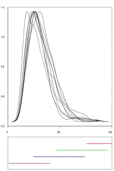
Figure 9: The ten distributions of size 500 samples (top) and the Euclidean cluster ranges (bottom)
(a) TRI (b) K25
(c) K50 (d) K95 (e) K95 (size 100 sample)
Figure 10: The FPs and cluster ranges for sample size 500: (a), (b), (c), (d), (e) cluster ranges for sample size 100 and the K95 FP
The ten sample distributions are plotted at the top of Figure 9, and the extrema of the cluster ranges, calculated over the ten runs, are plotted at the bottom. The five pseudo-metrics include the Euclidean distance and four FP-based pseudo-metrics corresponding to the FP shown in Figure 10. The cluster ranges are also plotted in Figure 10 below each corresponding FP.
We discuss these plots as follows. When the Euclidean distance is used in the hierarchical clustering, the process is completely unsupervised. The cluster bounds depend only on the number of groups and the data distribu- tion for each run, and it is difficult to interpret them. With the FP-based pseudo-metrics, the results are different. The cluster composition reflects the knowledge represented by the FP, almost strictly for the K95 partition, and with more flexibility for the K25, K50 or T RI partitions. For all FPs, the extrema of the cluster bounds are located within the corresponding MF sup- port range, reflecting the constraint that individuals belonging to the same concept are closer than those belonging to different MFs.
Table 2 summarizes the variances of the lower and upper bounds of the four clusters for each of the five pseudo-metrics.
Table 2: Variances of min and max cluster bounds, sample size: 500
Cluster
Euclidean Partition
Tri K25 K50 K95
min-max min-max min-max min-max min-max
1 1 45 1 14 1 7 1 1 1 0
2 47 129 14 48 6 22 1 15 0 0
3 193 110 52 55 22 26 16 20 0 0
4 558 219 81 219 54 219 34 219 3 219
Table 2 exhibits a clear trend: the wider the MF kernels, the smaller is the cluster bound variance. The K95 experiment is an extreme case. This config- uration drastically reduces the degree of freedom of the clustering algorithm, but it also highlights the importance of the distance parameter.
The means of the cluster counts for sample size 500 are given in Table 3.
The counts for theK95 FP may be used as a reference because this partition is close to a crisp partition. For this partition, the groups are unbalanced;
few items fall in the first and the fourth cluster. This unbalance is logical because the data distribution is skewed (as shown in Figure 9). To some
extent, the use of an FP-based pseudo-metric introduces supervision into the clustering process.
Table 3: Means of the cluster counts for sample size 500
G En Tri K25 K50 K95
1 315 130 93 63 36
2 158 259 256 279 271
3 22 102 137 147 183
4 4 10 14 12 11
In contrast, when using the Euclidean distance, the two first groups are more numerous and the third one includes less individuals. There is no supervising effect and the data distribution is no longer reflected in the cluster composition.
However, we must be cautious regarding this point. This supervising effect remains valid under the condition that the data distribution spans the whole range of the FP. With a small sample size, certain distributions may lack items at the edge. In this case, the fourth group range may also be included in the third fuzzy set support, as is the case for the sample size 100, which is shown at the bottom of Figure 10(e). Results for sample sizes 200 and 1000 are comparable to the results given for sample size 500.
We could therefore consider that we have a semi-supervised behavior, with the FP serving as a reference only if data are available to enforce that reference.
The study raises significant questions about the relative importance of clustering algorithm parameters and data locations for the resulting clus- ters. It is well known that the distance function is a key parameter for such algorithms, including the k-means algorithm. For instance, input variables can be weighted within the distance function, and in that case, changing the weighting coefficient vector is likely to yield a different partition.
Furthermore, the K95 experiment illustrates the importance given to ex- pert knowledge. In the case studies, partitions that are more realistic are used to introduce expert knowledge into the clustering procedure. Thus, ex- pert knowledge does not entirely define the clustering result, even more so in a multidimensional clustering procedure. To summarize, the results are dependent on the data and are biased by the FPs.
4.4. Real-world case study
To demonstrate the value of the proposed univariate pseudo-metric, this section presents a real-world application involving geographical data and ex- pert knowledge for decision support in wine growing.
The georeferenced data are yield data [25] from an embedded sensor on a grape-harvesting machine. The 1.4-ha field was planted with theBourboulenc variety and was harvested in 2001 in Provence (France). The average sam- pling rate is approximately 2400 measurements per ha. However, because of a data acquisition problem, some records are missing. A recurrent charac- teristic of many agro-environmental data is their lack of regularity because of missing data and manual measurement.
The objective of the study is to identify suitable management zones based on the information found in the yield data and the domain knowledge. Sev- eral operations could then be adapted, including fertilization, winter pruning and grassing.
An algorithm that is able to process data that are not necessarily on a regular grid is used. This algorithm is derived from a region-merging algo- rithm, and details about the algorithm can be found in [21]. A fundamental point is the way the spatial coordinates are used here. They are not directly involved in any dissimilarity calculation but are only used to define point and zone neighborhoods. The algorithm works on two spaces simultaneously (attribute space and geographic space). The proximity criterion used for zone merging is based on dissimilarity in the attribute space and is calcu- lated only within a given neighborhood. Spatial interpolation of data is not necessary for the algorithm to run, which is an asset because synthetic data are made by interpolation, and the artificial nature of these data is often not considered in the interpretation of the results.
The study compares the results obtained by running the algorithm with a Euclidean distance-based merging criterion and with an FP-based distance criterion. The FP is determined from local policy norms, and the fuzzy set breakpoints are 7,9,11. A FisPro [12] screenshot displaying the FP together with the data distribution is shown in Figure 11.
The algorithm yields a series of maps with a decreasing number of zones.
The six zone maps are shown in Figure 12-a and 12-b.
The main difference between the two maps is the presence of a north-south structure in the FP-based map, which does not appear in the other map. Two main management zones are highlighted in 12-b, one corresponding to the
Figure 11: Histogram and FP for the yield data
northern low yield and one corresponding to the southern high yield. From an expert point of view, this makes sense. Inversely, the absence of structure in Figure 12-a is derived from the fact that, with the Euclidean distance, medium-high yield data in the south-east have been associated with lower yield data to form zone #6 (in light gray).
A few specific zones of small size appear equally in both maps. These zones correspond to i) a zone of high yield in the center of the plot (zone #1, in black) and ii) a few low-yield zones located along the southern edge of the field, which correspond to border effects (beginning of the rows). Depending on the goal and the machinery of the grower, these small zones may not be considered for site-specific management.
The introduction of the FP-based pseudo-metric in the zoning method provides a map that simplifies the representation of the field, according to expert knowledge, while preserving the main trends found in the available data.
In many real-world applications, multidimensional data are to be consi- dered. We now propose a method for using FP-based pseudo-metrics in a multivariate framework.
a) Euclidean distance b) FP-based pseudo-metric
Figure 12: Zoning yield data with two types of distance
5. The multivariate case: a pseudo-metric and a case study
The easiest way to obtain a multidimensional pseudo-metric is to per- form a Minkowski-like combination of the univariate pseudo-metrics. Let two multidimensional points x = (x1, . . . , xM) and y = (y1, . . . , yM) with xi, yi ∈[0,1], ∀i∈1, . . . , M.
We have the following definition for the pseudo-metric:
∀x, y d(x, y) =
" M X
j=1
(dj(xj, yj))k
#1k
(13) In Equation (13), each dj is a univariate distance in the jth dimension, eitherdP as defined in Equation (5), which is based on a FPP, or a different univariate distance, for instance, a univariate Euclidean distance.
Because d(x, y) is a sum of semi-distance functions, it automatically in- herits the properties of a semi-distance.
For k=2 and regular SFPs in all dimensions, Equation (13) yields the same result as the multidimensional Euclidean distance.
Case study
Data chosen to demonstrate the value of the approach are taken from [15]
and have been used previously to illustrate clustering procedures [7]. The data set describes the percentages of water, protein, fat, lactose and ash in the milk of 22 mammals. Data are given in Table 4.
The aim of our case study is to cluster the mammals, according to these five milk components, by introducing FP-based pseudo-metrics into a clas- sical clustering procedure. First, a dissimilarity matrix between all pairs of items is computed. Then, the dissimilarity matrix is used as an input to the clustering algorithm. Because the standard k-means does not give stable results with the Euclidean distance, a robust version, called pam (partition- ing around medoids)[17], is used. The main difference between pam and k-means is the definition of the cluster centers: in the robust version, the cluster centers are not computed as the mean but are necessarily data items, in a formation called a medoid. The R implementation[23] of pam is used in the experiments.
Table 4: Ingredients of mammals milk
Water Protein Fat Lactose Ash Bison 86.90 4.80 1.70 5.70 0.90 Buffalo 82.10 5.90 7.90 4.70 0.78 Camel 87.70 3.50 3.40 4.80 0.71 Cat 81.60 10.10 6.30 4.40 0.75 Deer 65.90 10.40 19.70 2.60 1.40 Dog 76.30 9.30 9.50 3.00 1.20 Dolphin 44.90 10.60 34.90 0.90 0.53 Donkey 90.30 1.70 1.40 6.20 0.40 Elephant 70.70 3.60 17.60 5.60 0.63 Fox 81.60 6.60 5.90 4.90 0.93 Guinea Pig 81.90 7.40 7.20 2.70 0.85 Hippo 90.40 0.60 4.50 4.40 0.10 Horse 90.10 2.60 1.00 6.90 0.35 Llama 86.50 3.90 3.20 5.60 0.80 Monkey 88.40 2.20 2.70 6.40 0.18 Mule 90.00 2.00 1.80 5.50 0.47 Orangutan 88.50 1.40 3.50 6.00 0.24 Pig 82.80 7.10 5.10 3.70 1.10 Rabbit 71.30 12.30 13.10 1.90 2.30 Rat 72.50 9.20 12.60 3.30 1.40 Reindeer 64.80 10.70 20.30 2.50 1.40 Seal 46.40 9.70 42.00 0.00 0.85 Sheep 82.00 5.60 6.40 4.70 0.91 Whale 64.80 11.10 21.20 1.60 0.85 Zebra 86.20 3.00 4.80 5.30 0.70
Using the Euclidean distance
The results of thepampartitioning run on the multidimensional data are shown in Figure 13, which is a two-dimensional plot. The three clusters are labeled E1, E2, E3.
All observations are represented by points in the plot, and principal com- ponents analysis (PCA) is used to reduce the dimensions to the two first axes. An ellipse is drawn around each cluster. The first two components of the PCA explain 94.91% of the variability, and we will study the cluster composition on the first plane, also called the principal plane. Of course, some individuals may be closer or farther on the other factorial planes.
The cluster composition is somewhat unexpected. Dog is included in the cluster of sea mammals, whereas cat and pig are assigned to a different cluster.
−4 −2 0 2
−3−2−10123
Component 1
Component 2
●
● ●
●
●
●
● ●
●
●
Bison
Buffalo Camel
Deer Cat
Dog
Dolphin
Donkey
Elephant Fox Guinea Pig
Hippo Horse Llama
Monkey Mule
Orangutan Pig
Rabbit
Rat Reindeer
Seal
Sheep
Whale
Zebra 1
2
3
E E
E
% inertia: 76.2
% inertia: 18.7
Figure 13: Clusters obtained with the Euclidean distance
A powerful indicator can be computed using the silhouette index [24]. To construct the silhouettes S(i) for each item i, the following formula is used:
S(i) = b(i)−a(i) max(a(i), b(i))