Generic Polar Harmonic Transforms for Invariant Image Representation
Thai V. Hoang∗,1 and Salvatore Tabbone2
1Inria Nancy-Grand Est, 54600 Villers-l`es-Nancy, France
2Universit´e de Lorraine, LORIA, 54506 Vandœuvre-l`es-Nancy, France
Abstract
This paper introduces four classes of rotation-invariant orthogonal moments by generalizing four existing moments that use harmonic functions in their radial kernels. Members of these classes share beneficial properties for image representation and pattern recognition like orthogonality and rotation-invariance. The kernel sets of these generic harmonic function-based moments are complete in the Hilbert space of square-integrable continuous complex-valued functions. Due to their resemble definition, the computation of these kernels maintains the simplicity and numerical stability of existing harmonic function-based moments. In addition, each member of one of these classes has distinctive properties that depend on the value of a parameter, making it more suitable for some particular applications. Comparison with existing orthogonal moments defined based on Jacobi polynomials and eigenfunctions has been carried out and experimental results show the effectiveness of these classes of moments in terms of representation capability and discrimination power.
Keywords: Polar harmonic transforms; harmonic kernels; rotation invariance; orthogonal moments
1 Introduction
Rotation-invariant features of images are usually extracted by using moment methods [1] where an imagef on the unit disk (x2+y2 ≤1) is decomposed into a set of kernels {Vnm|(n, m)∈Z2} as
Hnm= Z Z
x2+y2≤1
f(x, y)Vnm∗ (x, y) dxdy,
where the asterisk denotes the complex conjugate. According to [2], a kernel that is “invariant in form”
with respect to rotation about the origin must be defined as Vnm(r, θ) =Rn(r)Am(θ), where r = p
x2+y2, θ = atan2(y, x), Am(θ) = eimθ, and Rn could be of any form. For example, rotational moments (RM) [3] and complex moments (CM) [4] are defined by using Rn(r) = rn; continuous generic Fourier descriptor (GFD) [5] employs ei2πnr forRn(r); and angular radial transform (ART) [6] uses harmonic functions as
Rn(r) =
(1, n= 0 cos(πnr), n6= 0.
∗Corresponding author
E-mail address: vanthai.hoang@inria.fr,Telephone: +33 3 54 95 85 60,Fax: +33 3 83 27 83 19.
However, the obtained kernelsVnm of RM, CM, GFD, and ART are not orthogonal and, as a result, information redundancy exists in the momentsHnm, leading to difficulties in image reconstruction and low accuracy in pattern recognition, etc. Undoubtedly, orthogonality between kernelsVnm comes as a natural solution to these problems. Orthogonality means
hVnm, Vn0m0i= Z Z
x2+y2≤1
Vnm(x, y)Vn∗0m0(x, y) dxdy
= Z 1
0
Rn(r)R∗n0(r)rdr Z 2π
0
Am(θ)A∗m0(θ) dθ=δnn0δmm0,
where δij = [i=j] is the Kronecker delta function. It can be seen from the orthogonality between the angular kernels
Z 2π 0
Am(θ)A∗m0(θ) dθ= Z 2π
0
eimθe−im0θdθ= 2πδmm0 that the remaining condition on the radial kernels is
Z 1 0
Rn(r)R∗n0(r)rdr= 1
2πδnn0. (1)
This equation presents the regulating condition for the definition of a set of radial kernels Rn in order to have orthogonality between kernelsVnm.
There exists a number of methods that have their radial kernels satisfying the condition in Eq. (1) and they can be roughly classified into three groups. The first employsJacobi polynomials [7] inr of ordernfor Rn(r) obtained by orthogonalizing sequences of polynomial functions or by directly using existing orthogonal polynomials. Members of this group are Zernike moments (ZM) [8], pseudo-Zernike moments (PZM) [2], orthogonal Fourier–Mellin moments (OFMM) [9], Chebyshev–Fourier moments (CHFM) [10], and pseudo Jacobi–Fourier moments (PJFM) [11] (see [12, Section 6.3], or [13, Section 3.1] for a comprehensive survey). It was demonstrated recently that the Jacobi polynomial-based radial kernels of these methods are special cases of the shifted Jacobi polynomials [14,15]. Despite its popularity, this group of orthogonal moments however involves computation of factorial terms, resulting in high computational complexity and numerical instability, which often limit their practical usefulness.
The second group employs theeigenfunctions of the Laplacian∇2 on the unit disk asVnm, similar to the interpretation of Fourier basis as the set of eigenfunctions of∇2 on a rectangular domain. These eigenfunctions are obtained by solving the Helmholtz equation,∇2V +λ2V = 0, in polar coordinates to have the radial kernels defined based on the Bessel functions of the first and second kinds [16]. In addition, by imposing the condition in Eq. (1) a class of orthogonal moments is obtained [17] and different boundary conditions were used for the proposal of a number of methods with distinct definition ofλ:
Fourier–Bessel modes (FBM) [18], Bessel–Fourier moments (BFM) [19], and disk-harmonic coefficients (DHC) [20]. However, the main disadvantage of these eigenfunction-based methods is the lack of an explicit definition of their radial kernels other than Bessel functions, leading to inefficiency in terms of computation complexity.
And the last group uses harmonic functions (i.e., complex exponential and trigonometric functions) forRn by taking advantage of their orthogonality:
Z 1 0
ei2πnre−i2πn0rdr=δnn0, (2)
Z 1 0
cos(πnr) cos(πn0r) dr= 1
2δnn0, (3)
Z 1
0
sin(πnr) sin(πn0r) dr= 1
2δnn0, (4)
Z 1 0
cos(πnr) sin(πn0r) dr= 0, n−n0 is even, (5) It can be seen that the integrand in Eqs. (2)–(5) is “similar in form” with that in Eq. (1), except for the absence of the weighting termr which prevents a direct application of harmonic functions as radial kernels. This obstacle was first overcome in [21] by using the multiplicative factor √1r in the radial kernels to eliminater in the definition of radial harmonic Fourier moments (RHFM) as
Rn(r) = 1
√r
1, n= 0
√
2 sin(π(n+ 1)r), n >0 & nis odd
√
2 cos(πnr), n >0 & nis even.
(6)
Recently, a different strategy was proposed to mover into the variable of integration,rdr= 12dr2, in the definition of three different forms of polar harmonic transforms[22]: polar complex exponential transform (PCET), polar cosine transform (PCT), and polar sine transform (PST). The radial kernels of these transforms are respectively defined as
Rn(r) = ei2πnr2, (7)
RCn(r) =
(1, n= 0
√2 cos(πnr2), n >0 (8)
RSn(r) =
√
2 sin(πnr2), n >0 (9)
It is straightforward that the radial kernels in Eqs. (6)–(9) all satisfy the orthogonality condition in Eq. (1) and that their corresponding kernels are orthogonal over the unit disk. In addition, the radial kernels of RHFM in Eq. (6) are actually equivalent toRn(r) = √1rei2πnr in terms of image representation, similar to the equivalence between different forms of Fourier series (namely trigonometric and complex exponential functions). The resemblance between the exponential form of RHFM’s radial kernels and PCET’s radial kernels suggests that they are actually special cases of a generic class of radial kernels that are defined based on complex exponential functions. And each member of this class can be used to define kernels that are orthogonal over the unit disk. Similar observation also leads to generic classes of radial kernels defined based on trigonometric functions.
The main contribution of this paper is a generic view on strategies that were used to define orthogonal moments. This leads to the introduction of four classes of radial kernels that correspond to four generic sets of moments and take existing harmonic moments as special cases. This paper proves theoretically that the generic sets of kernels are complete in the Hilbert space of all square-integrable continuous complex-valued functions over the unit disk. It also shows experimentally that the proposed harmonic moments are superior to Jacobi polynomial-based moments and are comparable to eigenfunction-based moments in terms of representation capability and discrimination power. It is also interesting to note that these generic harmonic moments can be computed very quickly by exploiting the recurrence relations among complex exponentials and trigonometric functions [23]. The generalization by introducing a parameter in this paper is similar to the generalization of theR-transform published recently[24].
The content of this paper is a comprehensive extension of the research work presented previously in [25]. The next section will derive explicit form of generic classes of radial kernels defined based on complex exponentials and trigonometric functions. The completeness of the sets of orthogonal decomposing kernels is proven in Section3, along with some beneficial properties obtained from the
generalization. Section4 is devoted to the stability of the numerical computation. Experimental results in terms of representation capability and discrimination power are given in Section5. And conclusions are finally drawn in Section 6.
2 Generic polar harmonic transforms
In order to formulate the generalization, assuming that the harmonic radial kernels have the generic exponential formRns(r) =κ(r) ei2πnrs, where s∈Rand κ is a real functional of r. Then
Z 1 0
Rns(r)R∗n0s(r)rdr = Z 1
0
κ2(r) ei2πnrse−i2πn0rsrdr.
Since drs =srs−1dr =srs−2rdr then Z 1
0
Rns(r)Rn∗0s(r)rdr= Z 1
0
κ2(r)
srs−2 ei2πnrse−i2πn0rsdrs. By letting srκ2s−2(r) = const =C,
Z 1 0
Rns(r)R∗n0s(r)rdr= Z 1
0
Cei2πnrse−i2πn0rsdrs=Cδnn0.
In order to have orthonormality between kernels, it follows directly from Eq. (1) thatC= 2π1 . Then κ(r) =
qsrs−2
2π and Rns have the following actual definition:
Rns(r) =κ(r) ei2πnrs, (10)
or
Vnms(r, θ) =Rns(r)Am(θ) =κ(r) ei2πnrseimθ. (11) The generic polar complex exponential transform (GPCET) is thus defined as
Hnms = Z Z
x2+y2≤1
f(x, y)Vnm∗ (x, y) dxdy= Z 2π
0
Z 1 0
f(r, θ)κ(r) e−i(2πnrs+mθ)rdrdθ. (12)
By considering s in the above development as a parameter, it can be seen that Rns is a true generalization of the harmonic radial kernels of PCET [22]: Rns(r) in Eq. (10) becomesRn(r) in Eq.
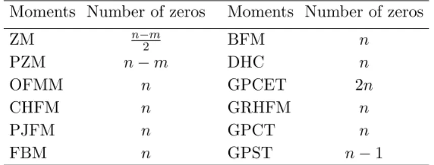
(7) when s = 2, except for the constant multiplicative factor √1π. Thus, a class of harmonic radial kernels can be obtained by changing the value ofs. Due to the generic definition, members of this class share beneficial properties to image representation and pattern recognition. However, each member also possesses distinctive characteristics that are determined by the actual value ofs, making it more suitable for some particular applications. Some beneficial properties of GPCET will be discussed in Section3 and be supported by experimental evidence in Section5. Figure 1 illustrates the phase of GPCET kernels using four different values ofs= 0.5,1,2,4 for{(n, m)|n, m∈[0,2],(n, m)∈Z2}. It can be seen that the phase of Vnms, unlike that of the kernels defined based on polynomials, is the sum of the phase ofRns andAm. The phase image ofVnms thus has a rotational symmetry pattern composing of repetitive slices whenn or m6= 0. The dependence of this pattern on n, m, and scan be described as follows:
- an increase inn results in thinner and longer slices.
m= 0 m= 1 m= 2
n=0n=1n=2
(a)s= 0.5
m= 0 m= 1 m= 2
n=0n=1n=2
(b)s= 1
m= 0 m= 1 m= 2
n=0n=1n=2
(c)s= 2
m= 0 m= 1 m= 2
n=0n=1n=2
(d)s= 4
Figure 1: 2D view of the phase of GPCET kernels Vnms defined in Eq. (11) using s= 0.5,1,2,4 for {(n, m)|n, m∈[0,2],(n, m)∈Z2}. In each figure (i.e., for a specific value ofs), the row and column indices indicate the values ofn= 0,1,2 (top to bottom) andm= 0,1,2 (left to right), respectively.
- an increase inm increases the number of slices.
- a change ins corresponds to a change in the thickness uniformity of each slice.
In addition to the harmonic radial kernels of GPCET defined in Eq. (10), there exist three other classes of harmonic radial kernels that result from generalizing the harmonic radial kernels of RHFM (RnsH) [21], PCT (RCns), and PST (RSns) [22]. By using similar development procedures, it is straightforward that
RHns(r) =κ(r)
1, n= 0
√2 sin(π(n+ 1)rs), n >0 & nis odd
√2 cos(πnrs), n >0 & nis even
(13)
RCns(r) =κ(r)
(1, n= 0
√2 cos(πnrs), n >0 (14)
RSns(r) =κ(r)
√
2 sin(πnrs), n >0. (15)
These three classes of harmonic radial kernels correspond to three classes of transforms: the generic radial harmonic Fourier moments (GRHFM), the generic polar cosine transforms (GPCT), and the generic polar sine transforms (GPST). GRHFM is in fact a variant of GPCET in terms of representation, similar to the equivalence between different forms of Fourier series. It becomes RHFM in Eq. (6) when s= 1, except for the constant multiplicative factor √1
2π. In addition, GPCT/GPST arise naturally from GRHFM when the function to be represented by RHns is considered as half of an even/odd periodic function. Again, GPCT/GPST become PCT/PST in Eqs. (8)/(9) whens= 2, except for the constant multiplicative factor √1π.
Orthogonal sets
At a specific value ofs,hVnms, Vn0m0si=δnn0δmm0 means that
Bs ={Vnms(r, θ) =Rns(r) eimθ |n, m∈Z} (16) forms a set of kernels that are orthonormal over the unit disk. Similarly, there are three other sets of orthonormal kernels at a specific value of sdefined as
BsH ={VnmsH (r, θ) =RnsH(r) eimθ |n∈N, m∈Z}, (17)
BCs ={VnmsC (r, θ) =RnsC(r) eimθ |n∈N, m∈Z}, (18) BsS ={VnmsS (r, θ) =RnsS (r) eimθ |n∈Z+, m∈Z}. (19) Each of the setsBs, BHs , BsC, and BsS can be used as the set of decomposing orthonormal kernels for GPCET, GRHFM, GPCT, and GPST, respectively. The completeness of these sets is an important issue that needs further consideration (see Section3).
In spite of their common harmonic nature, each of GPCET, GRHFM, GPCT, and GPST captures different image information even at the same value ofs, similar to the difference among Fourier (complex exponential and trigonometric), cosine, and sine series. This observation will have experimental evidence in Section5. Nevertheless, in the remaining of this paper, the theoretical discussions will mainly focus on GPCET with an occasional foray into GRHFM, GPCT, and GPST only when necessary. This is to avoid unnecessary repetition, since GRHFM, GPCT, and GPST essentially have many properties that are identical to those of GPCET. In addition, if not explicitly mentioned, the parameterswill have a fixed value in the remaining discussions.
3 Properties
This section discusses the completeness of the sets of orthogonal decomposing kernels defined in Eq. (16) along with some beneficial properties of GPCET for image representation and pattern recognition that result directly from the generalization. Other issues like relation with RM, 3D formulation, rotation invariance, rotating-angle estimation, and computational complexity could also be derived with relative ease [13, Section 3.3].
3.1 Completeness of Bs
A set of orthogonal kernels is called complete in a Hilbert space Hif its linear span is dense inH. The completeness of an orthogonal set inHis hence related to the ability of the set in representing functions inH. In the case of Bs,H is defined as the space of all square-integrable continuous complex-valued functions over the unit disk, denoted asL2(x2+y2 <1). A completeBs can be used as an orthonormal basis, meaning that every functionf ∈ H can be written as an infinite linear combination of the kernels inBs as
fs(x, y) =
∞
X
n=−∞
∞
X
m=−∞
HnmsVnms(x, y). (20)
In addition, due to the Parseval’s identity:
X
(n,m)∈Z2
|Hnms|2= Z Z
x2+y2≤1
|f(x, y)|2dxdy,
it can be seen that GPCET moments,Hnms, are bounded if and only if f is square-integrable. The above identity is in fact stronger than the Bessel’s inequality claimed in [22, Eq. (8)], where a loose inequality is used instead of an equality. This is because [22] lacks discussion on the completeness of its proposed orthogonal sets.
In this subsection, the completeness of Bs in H is established by means of the interpretation of GPCET through Fourier series by rewriting Eq. (12) as
Hnms= Z 2π
0
Z 1 0
f(r, θ)κ(r) e−i2πnrsrdr
e−imθdθ= 1 2π
Z 2π 0
Z 1 0
g(r0, θ) e−i2πnr0dr0
e−imθdθ,
wherer0=rs and
g(r0, θ) = r2π
s r02−s2s f s
√ r0, θ
. (21)
If g is viewed as a 2D function defined in a Cartesian coordinate system where r and θ are the horizontal and vertical axes, respectively, then the GPCET moments Hnms of a functionf ∈ H are the 2D Fourier coefficients of gformulated as above: first in the radial direction, then in the angular direction. This interpretation transforms the completeness issue ofBs inH into the convergence issue of 2D Fourier series, leading to the following two questions:
- The convergence of partial sums of 2D Fourier series of functions? Almost everywhere convergence of “polygonal partial sums” of 2D Fourier series of functions in L2([0,1]×[0,2π)) was already established in [26].
- The square-integrability ofg? The necessary and sufficient conditions for the square-integrability ofg over the domain [0,1]×[0,2π) will be established in Theorem1.
Theorem 1. The function g defined in Eq.(21) is in L2([0,1]×[0,2π)) if and only if the function f is in L2(x2+y2<1).
Proof. From the definition of g:
Z 2π 0
Z 1 0
|g(r0, θ)|2dr0dθ= Z 2π
0
Z 1 0
2π
s r02−ss f s
√ r0, θ
2dr0dθ.
By changing the variable r=√s
r0 →r0 =rs and dr0=srs−1dr, the above equation becomes Z 2π
0
Z 1
0
|g(r0, θ)|2dr0dθ= Z 2π
0
Z 1
0
2π
s r2−s|f(r, θ)|2srs−1drsdθ
= 2π Z 2π
0
Z 1
0
|f(r, θ)|2rdrdθ= 2π Z Z
x2+y2≤1
|f(x, y)|2dxdy.
Thus, it is straightforward that Z 2π
0
Z 1 0
|g(r0, θ)|2dr0dθ <∞ ⇔ Z Z
x2+y2≤1
|f(x, y)|2dxdy <∞
and the theorem is proven.
Thus, the set Bs= {Vnms |n, m ∈Z} is complete in the Hilbert spaceH of all square-integrable continuous complex-valued functions over the unit diskL2(x2+y2 <1). As a result, Bs can be used as an orthonormal basis forHand writingf as in Eq. (20) is safe (i.e., the partial sums converge to the image function). To our knowledge, there exists no such conclusion for other orthogonal sets over the unit disk where the corresponding radial kernels are defined based on polynomials or eigenfunctions.
3.2 Zeros of Rns
The number of zeros of the radial kernels is an important indicator since it corresponds to the capability of moments in representing high frequency components of images. In the case of GPCET,Rnsis defined based on complex exponential function and can be rewritten in the following form:
Rns(r) =κ(r) h
cos(2πnrs) +isin(2πnrs) i
,
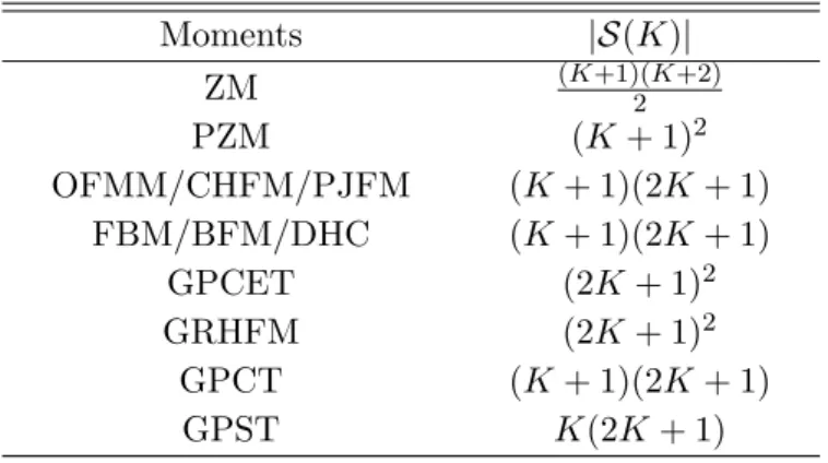
Table 1: The number of zeros of the nth-order radial kernel of existing unit disk-based orthogonal moments.
Moments Number of zeros Moments Number of zeros
ZM n−m2 BFM n
PZM n−m DHC n
OFMM n GPCET 2n
CHFM n GRHFM n
PJFM n GPCT n
FBM n GPST n−1
and the two equations
real(Rns(r)) = 0, imag(Rns(r)) = 0
both have 2ndistinct roots in the interval 0< r <1. For a better perception of how large this number is, Table1provides the number of zeros of thenth-order radial kernel of existing unit disk-based orthogonal moments. It can be seen that, except for ZM, PZM, and GPCET, thenth-order radial kernel of all other methods has approximatelyn zeros. In the case of GPCET, this number is almost double whereas, for ZM and PZM, it depends on the angular orderm. In order to have the same number of zerosn0 as other methods, the order of the radial kernel of ZM and PZM has to be 2n0+m and n0+m, respectively.
These numbers are much higher than that of GPCET, which is only n20.
In addition to the quantity, the distribution of zeros is also an important property of the radial kernels since it relates to theinformation suppression problem [4]. Suppression is the situation when the computed moments put emphasis on certain portions of image and neglect the rest. When the essential discriminative information is distributed uniformly over the image domain, an unfair emphasis of the extracted moments is known to have a negative impact on their discrimination power. On the contrary, when the essential discriminative information only exists in certain image portions, it is preferable to move the emphasis towards those portions. In the case of GPCET, the distribution of the zeros ofRns
can be controlled by changing the parameter s. In other words, emphasis can be put on the image portions that contain this information. This is the distinctive property of GPCET that existing methods do not have.
When s= 1, the zeros of Rn1 are distributed uniformly, meaning a uniform emphasis over the image region. The more deviation of the value of sfrom 1 is, the more “biased” to the inner (whens <1) or outer (whens >1) portions of the unit disk the distribution of zeros is. This in turn corresponds to the more emphasis on the inner or outer portions of image, respectively. Evidence for the observations on the quantity and distribution of zeros of Rns is given in Figure2 that contains the plot of real(Rns) and imag(Rns) of orders n= 0→4 ats= 0.5,1,2,4 (top row to bottom row). It can be seen that the real and imaginary parts of GPCET radial kernel of order nhave 2n zeros in the interval 0< r <1.
Moreover, the distribution of these zeros is biased towards 0 ats= 0.5, uniform at s= 1, and biased towards 1 ats= 2,4.
4 Numerical stability
Accuracy is another concern when moments are computed numerically. Error in the computed moments may result from the discrete approximation of continuous mathematical formulas or from the digital
0 0.2 0.4 0.6 0.8 1
−4
−2 0 2 4
real(Rns(r))
r
n= 0 n= 1 n= 2 n= 3 n= 4
0 0.2 0.4 0.6 0.8 1
−4
−2 0 2 4
imag(Rns(r))
r
n= 0 n= 1 n= 2 n= 3 n= 4
0 0.2 0.4 0.6 0.8 1
−2
−1 0 1 2
real(Rns(r))
r
n= 0 n= 1 n= 2 n= 3 n= 4
0 0.2 0.4 0.6 0.8 1
−2
−1 0 1 2
imag(Rns(r))
r
n= 0 n= 1 n= 2 n= 3 n= 4
0 0.2 0.4 0.6 0.8 1
−0.5 0 0.5
real(Rns(r))
r n= 0
n= 1 n= 2 n= 3 n= 4
0 0.2 0.4 0.6 0.8 1
−0.5 0 0.5
imag(Rns(r))
r n= 0
n= 1 n= 2 n= 3 n= 4
0 0.2 0.4 0.6 0.8 1
−1 0 1
real(Rns(r))
r n= 0
n= 1 n= 2 n= 3 n= 4
0 0.2 0.4 0.6 0.8 1
−1 0 1
imag(Rns(r))
r n= 0
n= 1 n= 2 n= 3 n= 4
Figure 2: Real and imaginary parts of GPCET radial kernels of ordersn= 0→4 ats= 0.5,1,2,4. The real and imaginary parts of GPCET radial kernel of order nhave 2n zeros in the interval 0< r <1.
The distribution of these zeros is uniform when s= 1 and biased towards 0 or 1 depending on whether s <1 or s >1.
nature of computing systems, where numbers can only be represented in a certain range and to a certain precision. In addition, error also has its root in the mathematical definition of moments. These two error sources and their impacts will be discussed in the remaining of this section.
4.1 Approximation error
Since moments are originally defined based on a double continuous integral over the unit disk domain, the following discrete approximation of Eq. (12) will incur error in the computed moments:
Hnms= X
[i,j]∈C
f(xi, yj)Vnms∗ (xi, yj)∆x∆y, (22) where C is the set of pixels whose mapped regions lie entirely inside the unit disk; (xi, yj) are the coordinates of the center of the mapped region of pixel [i, j]; and ∆x and ∆y are the dimensions of each mapped region. In the above equation, there are two types of discrete approximations and they correspond to two types of approximation errors [27]: geometric error and numerical error. Geometric error occurs when the domain of integration does not exactly cover the unit disk, due to the difference between circular and rectangular domains. This type of error, however, could be “avoided” if only the pixels that lie entirely inside the unit disk are used and the image function over the remaining regions
of the unit disk is assumed to take value 0. Since this strategy will be used for the computation of harmonic function-based moments and comparison methods, geometric error hence does not exist in all experiments in Section 5.
Numerical error arises when Vnms∗ (xi, yj)∆x∆y in Eq. (22), which represents the value of the kernel Vnms over the pixel [i, j], is computed by a numerical integration technique. Since the numerically computed value of Vnms∗ (xi, yj)∆x∆y is just an approximation to its analytical value, this type of error cannot be avoided in any way if one chooses to compute moments by numerical approximation. The magnitude of this type of error, however, could be reduced if only a highly accurate numerical integration technique is employed (e.g., “pseudo” sub-sampling or cubature). It can be seen from the factor ∆x∆y that the effect of numerical error depends on image size: a smaller-sized image will have a more severe effect, and vice versa. The effect of numerical error on harmonic function-based moments and comparison methods will be demonstrated experimentally by means of reconstruction error in Section5.
4.2 Representation error
In computing systems nowadays, a real number is in general approximately represented in floating-point format in order to allow reasonable storage requirement and relatively quick calculations. The typical number that can be represented exactly is of the form:
Significand×baseexponent,
where significand denotes a signed digit string of a given length in a given base and exponent is a signed integer which modifies the magnitude of the number. As computing systems are binary in nature, floating-point numbers are normalized for representation as ±(1 +f)×2e, wheref is the fraction or mantissa (0≤f <1) andeis the exponent. In 32-bit computers that use the IEEE 754 standard,double precision floating numbers occupy two storage locations, or 64 bits, to store the value off,e, and the sign:
52 bits forf, 11 bits fore+ 1023, and 1 bit for the sign. A double numbervthus can only be represented with the relative accuracy of one-half themachine epsilon, or 12×eps= 12×2−52'1.1102×10⁻¹⁶. This means that, when represented in the ordinary decimal numeral system, only the first 15 leftmost digits of vare significant. Because of the limited range ofe, the absolute values of double numbers are additionally limited in the range 2−1022÷(2−eps) 21023, or approximately 2.2251×10−308÷1.7977×10308. This finite set of double numbers with finite precision leads to the phenomena of underflow, overflow, androundoff in computing systems. Due to their nature, it is known in the literature that Jacobi polynomial-based methods suffer from all three types of errors [28] as pointed out below.
Underflow error occurs when an absolute value of a computed quantity (except zero) is under the range of its data type. Jacobi polynomial-based methods have this type of error due to the use of powers of r in their definition. At a radial coordinate r that is close to zero, let’s say r = 0.001, r102= 1.0000×10−306 andr103= 1.0000×10−309. Thus, any computation that involves r to the power greater than 102 will cause underflow error. It is obvious that this type of error depends on the size of images: a larger-sized image starts to have this error at a lower order. As an example, for an input image of size 1024×1024 pixels, the smallest value ofr in the computation is 10241 = 2−10= 9.7656×10⁻⁴, underflow error will start to occur atn= 103 onwards for all Jacobi polynomial-based methods.
Overflow error occurs when a computed quantity has a value above the range of its data type. Jacobi polynomial-based methods has this type of error due to the use of factorials in their definition. Since 170! = 7.2574×10306 and 171! = 1.2410×10309, any computation that involves factorial of a number greater than 170 will cause overflow error. From the definition of Jacobi polynomial-based radial kernels, it is straightforward that ZM, PZM, OFMM, CHFM, and PJFM start to have this type of error at n= 171,85,85,171,and 84 onwards, respectively.
Table 2: The radial orders of Jacobi polynomial-based methods from which underflow, overflow, and roundoff errors start to occur for an input image of size 1024×1024 pixels.
Error type ZM PZM OFMM CHFM PJFM
Underflow 103 103 103 103 103
Overflow 171 85 85 171 84
Roundoff 46 23 23 79 21
Roundoff error is the difference between an approximation of a number used in computation and its exact (i.e., correct) value. Because of the finite precision in computing systems, this type of error occurs in almost all numerical computation steps. However, Jacobi polynomial-based methods face the problem of large polynomial’s coefficients in their radial kernels. These coefficients are sometimes larger than 252 and thus, for the commonly 15-digit precision, computing radial kernels produces error of the order of unity or larger. It is not difficult to determine the order where each Jacobi polynomial-based method starts to have this type of error. They aren= 46,23,23,79,and 21 for ZM, PZM, OFMM, CHFM, and PJFM, respectively.
The starting orders for each type of error for all Jacobi polynomial-based methods are collected and given in Table2. Due to their distinct definition, it can be seen that different methods have different orders for overflow and roundoff errors. For underflow error, Jacobi polynomial-based methods have the same order because their radial kernels of the same order have the same polynomial order. Among these three types of representation errors, roundoff error occurs at the smallest order for each Jacobi polynomial-based method. Thus, roundoff error is the main concern in moment computation.
From the above definition of three types of representation errors, it can be seen that eigenfunction- based and harmonic function-based methods do not suffer from the underflow and overflow errors.
They do have roundoff error because of the nature of numerical computing systems. However, the effect of roundoff error on them is not as severe as on Jacobi polynomial-based methods because their definition does not use large-valued coefficients. In contrast, this effect causes serious problems in Jacobi polynomial-based methods, as will be shown experimentally in the next section. Nevertheless, any of the aforementioned error types is undesirable since it alters the computed values of moments, compromises the orthogonality of moments/kernels, and finally corrupts the overall performance of applications.
4.3 Singularity
In theory, GPCET could be defined as in Eq. (12) for everys∈R. However, because the multiplicative term is defined asκ(r) =
qsrs−2
2π , it should be aware that
s<2,r→0lim
rsrs−2
2π = +∞.
Evidence for this behavior can be seen in Figure 2for the casess= 0.5 and s= 1 where the magnitude of the real and imaginary parts of GPCET radial kernels go to infinity asr →0. These phenomena also exist in the other harmonic function-based methods and in CHFM. However, this property does not result in “big” problems because the actual computation is carried out by using Eq. (22), instead of Eq.
(12). As long as the center (xi, yj) of the pixel’s mapped region does not coincide (0,0), the computed moments are bounded and hence harmonic function-based methods withs <2 and CHFM can still be used for image representation and in pattern recognition problems. The practical usefulness of these methods will be demonstrated by experiments in the following section.
A B C D E F G H I J K L M N O P Q R S T U V W X Y Z
(a) Vector character images
(b) 16×16 (c) 32×32 (d) 64×64
(e) 128×128 (f) 256×256 (g) 512×512
Figure 3: (a) The vector character images used to generate six character datasets used in the recon- struction experiments by sampling these images to have the sizes of 16×16, 32×32, 64×64, 128×128, 256×256, and 512×512 pixels, corresponding to the six datasets. (b)-(g) Some sampled images from the six datasets.
5 Experimental results
The effectiveness of the proposed harmonic function-based moments will be demonstrated in comparison with existing moments of the same nature, i.e. unit disk-based orthogonal moments, through two types of experiments: image representation and pattern recognition. The first deals with the capability of harmonic function-based moments in representing pattern images and is done via image reconstruction.
The second is on the applicability of harmonic function-based moments in rotation-invariant pattern recognition problems at different levels of noise.
5.1 Image reconstruction and numerical stability
In the following experiments, a set of six character datasets has been generated by sampling 26 vector images of Latin characters in Arial bold font (shown in Figure3a) to have the sizes of 16×16, 32×32, 64×64, 128×128, 256×256, and 512×512 pixels. The purpose of using datasets of images of different sizes generated from the same source is to investigate the influence of numerical error discussed in Section4 on the computed values of moments of comparison methods. The representation error, which exists in Jacobi polynomial-based methods, will become apparent when moments of high-enough radial orders are involved. Some samples of reconstructed images from the character image “E” of size 64×64 pixels by GPCET are given in Figure4. The corresponding images of harmonic function-based (GPCET, GPCT, GPST), Jacobi polynomial-based (ZM, PZM, OFMM, CHFM, PJFM), and eigenfunction-based (FBM, BFM, DHC) methods are given in Figures 1 and 2 in the Supplemental material. In these figures, at each value ofK, all moment orders (n, m) that satisfy the conditions in Table3are used for reconstruction. These conditions are selected so that the moments that capture the lowest frequency information are used first in the reconstruction process.
Generally, as more moments are involved, the reconstructed images get closer to the original ones.
However, in the case of PZM, OFMM, and PJFM, reconstructed images deteriorate quickly atK = 23, 23, and 21 onwards, respectively. Similar phenomena also exist in other Jacobi polynomial-based methods but at a higher value ofK (46 for ZM and 79 for CHFM). Harmonic function-based methods
Table 3: The constraints on moment order nand repetitionm of comparison methods with regard toK.
Moments Order range
ZM |m| ≤n≤K,n− |m|= even
PZM |m| ≤n≤K
OFMM/CHFM/PJFM 0≤ |m|, n≤K
FBM/BFM/DHC 0≤ |m|, n≤K
GPCET |m|,|n| ≤K
GRHFM |m| ≤K, 0≤n≤2K
GPCT 0≤ |m|, n≤K
GPST |m| ≤K, 1≤n≤K
s=0.5s=1.0s=2.0s=4.0
Figure 4: Some samples of reconstructed images from the character image “E” of size 64×64 pixels by GPCET ats= 0.5,1,2,4 forK = 0,1, . . . ,29 (from left to right, top to bottom).
have difficulty in restoring the inner portion of the images whens= 2,4 with more difficulty ats= 4. On the contrary, they have difficulty with the images’ outer portion whens= 0.5. This is the experimental evidence for the information suppression problem mentioned in Subsection 3.2. Among harmonic function-based methods and at a specific value ofs, GPCET has better reconstructed images whenK is small. At high values ofK, images reconstructed by GPCT/GPST are closest/farthest to the original images at the corresponding values of K. This means that GPCT/GPST require the least/largest numbers of moments in order to reconstruct images of similar quality. These superiority/inferiority of GPCT/GPST can be easily observed at boundary regions wherer'0 andr '1. In addition, harmonic function-based and eigenfunction-based methods capture the image information, especially the edges, better than Jacobi polynomial-based methods. It thus can be concluded here that the more deviation the value ofsfrom 1 is, the more difficulty harmonic function-based methods will have to reconstruct the inner (whens >1) or outer (whens <1) portions of images. Conversely, harmonic function-based methods can reconstruct quickly the inner or outer portions of images whens <1 ors >1, respectively.
In other words, the parameters could be used to control the representation capability of harmonic function-based methods: more emphasis could be placed on certain regions of interest.
Table 4: The cardinality |S(K)|of the set S(K) = {(n, m) |n, m ∈ Z} of comparison methods at a specific value of K.
Moments |S(K)|
ZM (K+1)(K+2)2
PZM (K+ 1)2
OFMM/CHFM/PJFM (K+ 1)(2K+ 1)
FBM/BFM/DHC (K+ 1)(2K+ 1)
GPCET (2K+ 1)2
GRHFM (2K+ 1)2
GPCT (K+ 1)(2K+ 1)
GPST K(2K+ 1)
The gauge of reconstruction capability is measured by how well the reconstructed image is similar to the ground-truth one. For this purpose, the reconstruction error between an image and its reconstructed version is considered to be a good measure. In order to compute it, a finite set of moments is first calculated and then images are reconstructed from them in order to compute the errors. Since this process involves the computation of moment kernels both in the decomposition and then reconstruction steps, this measure can additionally be used for the investigation of the numerical stability of comparison methods. LetS(K) be the set containing all (n, m) that satisfy the conditions stated in Table 3 at a specific value ofK. Table4 provides the cardinality|S(K)|of S(K) of comparison methods. For an image functionf defined over the region{(x, y)∈R2 |x2+y2 ≤1}, its reconstructed version by using all moments of orders (n, m)∈ S(K) is defined as
fˆs(x, y) = X
(n,m)∈S(k)
HnmsVnms(x, y).
The reconstruction error, normalized by the total image energy, is then defined as
MSRE(K) = E
( RR
x2+y2≤1
h
f(x, y)−fˆs(x, y)i2
dxdy )
E (
RR
x2+y2≤1
f2(x, y) dxdy
) ,
whereE{·} is the expectation in ensemble averaging over the image set. In the literature, MSRE(K) is called the mean-square reconstruction error [3]. It is straightforward to show theoretically that 0≤MSRE(K)≤1. The lower (upper) bounds of MSRE(K) are reached when|S(K)|reaches its limits, or |S(K)| = 0 (∞). However, because of the numerical/representation errors and the unreachable theoretical point |S(K)|=∞, the statement 0≤MSRE(K)≤1 does not hold. Instead, it can only be asserted that MSRE(K)>0. In this experiment, a smaller value of MSRE(K) means the reconstructed image ˆfs is more similar to f or, in other words, a better reconstruction. In addition, by simple observation, MSRE(K) should have a smaller value when more moments are used in the reconstruction process, regardless of their orders.
The MSRE(K) curves of GPCET on the six character datasets at different values ofs= 0.1 : 0.1 : 6.0 in MATLAB’s notation are given in Figure5. The corresponding curves of all harmonic function-based methods are given in Figures 3–6 in the Supplemental material. At a specific value ofsin the horizontal axis in each of these figures, there is a MSRE(K) curve where the number of employed moments|S(K)|
0 2 4 6 0
500
1000
1500
s
|S(K)| MSRE(K)
0 0.2 0.4 0.6 0.8 1
(a) 16×16
0 2 4 6
0
500
1000
1500
s
|S(K)| MSRE(K)
0 0.2 0.4 0.6 0.8 1
(b) 32×32
0 2 4 6
0
500
1000
1500
s
|S(K)| MSRE(K)
0 0.2 0.4 0.6 0.8 1
(c) 64×64
0 2 4 6
0
500
1000
1500
s
|S(K)| MSRE(K)
0 0.2 0.4 0.6 0.8 1
(d) 128×128
0 2 4 6
0
500
1000
1500
s
|S(K)| MSRE(K)
0 0.2 0.4 0.6 0.8 1
(e) 256×256
0 2 4 6
0
500
1000
1500
s
|S(K)| MSRE(K)
0 0.2 0.4 0.6 0.8 1
(f) 512×512
Figure 5: MSRE(K) curves of GRHFM on the six character datasets at different values ofs. In each of these figures, at a specific value ofsin the horizontal axis, there is a MSRE(K) curve with the number of employed moments |S(K)|and MSRE(K) values illustrated as the ordinate and the color of the grid points having abscissas.
and the mean-square reconstruction error MSRE(K) are illustrated as the ordinate and the color of the grid points that have abscissas. The values of MSRE(K) which are outside the color display range [0,1]
is assigned the red color. A red color in MSRE(K) clearly means that the reconstructed image ˆfs does not reflect at allf. It can be seen from these figures that the color patterns in Supplementary Figure 3 are exactly the same as those in Supplementary Figure 4, suggesting that the reconstructed images by GPCET and GRHFM are the same. This provides experimental evidence for the equivalence between the radial kernels of GPCET and GRHFM that has been disclosed in Section2. For the purpose of representation and/or compression, GPCET and GRHFM moments can thus be used interchangeably without any change in performance. For this reason, in the remaining of this subsection on image reconstruction and numerical stability, GPCET can be used on behalf of GRHFM in discussions and comparisons with other methods. Among GPCET, GPCT, and GPST, a closer resemblance between the color patterns in Supplementary Figures 3 and 5 is observed. In addition, for a specific image size and at the corresponding abscissassand ordinates |S(K)|, MSRE(K) generally has its highest and lowest values in the case of GPST and GPCT, respectively. This means that GPCT and GPST generally have the highest and lowest representation power, respectively, among harmonic function-based methods. It should be noted that similar observations have also been seen in other applications. For example in compression, it turns out that cosine functions are much more efficient than the other functions.
For each harmonic function-based method and at a specific value of s, increasing the image size leads to a decrease in the values of MSRE(K) at the corresponding ordinates|S(K)|. This means that the reconstructed images ˆfs are more similar to the original onef. The difference between MSRE(K) at different image sizes indicates the existence of numerical error in the computed moments. This provides experimental evidence for the effect of image size on this type of error already mentioned in Subsection 4: a smaller image size will lead to a higher numerical error, and vice versa. However, a
0 500 1000 1500 0
0.2 0.4 0.6 0.8 1
|S(K)|
MRSE(K)
GPCET−0.5 GPCET−1 GPCET−2 GPCET−4 GPCT−0.5 GPCT−1 GPCT−2 GPCT−4 GPST−0.5 GPST−1 GPST−2 GPST−4
Figure 6: MSRE(K) curves of harmonic function-based methods (GPCET, GPCT, GPST) at s = 0.5,1,2,4 on the 64×64 character dataset.
small difference in MSRE(K) between image sizes 256 and 512 suggests that the effect of numerical error becomes negligible for large-sized images. In addition, for each harmonic function-based method and at a specific image size, changing the value ofsalso leads to a change in the values of MSRE(K) at the corresponding ordinates |S(K)|. The value of MSRE(K) decreases slowly when s has a too small or a too high value. This is due to the negligence of the extracted moments on certain portions of images as discussed in Subsection3.2. For better visualization and for the purpose of comparison, Figure 6illustrates MSRE(K) curves of harmonic function-based methods (GPCET, GPCT, GPST) at s= 0.5,1,2,4 on the 64×64 character dataset. These curves are plotted in the traditional 2D Cartesian coordinate system where the number of employed moments|S(K)|and the mean-square reconstruction error MSRE(K) are used as the abscissa and ordinate, respectively. The comparison results on the six character datasets are given in Figure 7 in the Supplemental material. From the six figures that correspond to the six character datasets, the above observations on harmonic function-based methods can be verified with relative ease.
Comparison of GPCET with Jacobi polynomial-based and eigenfunction-based methods using MSRE(K) curves computed from the 64×64 character dataset is given in Figure 7. The comparison results on the six character datasets are given in Figure 8 in the Supplemental material. It can be seen from the figure that numerical error causes MSRE(K) to take higher values at a smaller image size at the corresponding abscissas|S(K)|, similar to the phenomenon already observed in harmonic function-based methods. This provides another experimental evidence for the theoretical arguments on numerical error in Subsection 4.1: a smaller image size will lead to a higher numerical error, and vice versa. Numerical stability of Jacobi polynomial-based methods breaks down when K is increased up to a certain value. The quick deteriorations in the images reconstructed by Jacobi polynomial-based methods observed in Figure 2 in the Supplemental material are exhibited here by sudden upturns in their corresponding MSRE(K) curves atK = 46, 21, 23, and 23 for ZM, PZM, OFMM, and PJFH, respectively. MSRE(K) curve of CHFM breaks down later atK = 79 (not shown in the figure). These observations conform with the theoretical arguments on representation error in Subsection4.2. The starting values ofK that cause deteriorations here are equal to the starting radial orders that cause roundoff error in Jacobi polynomial-based methods given in Table 2. For large-sized images, except for GPCET ats= 4 and for the sudden upturn of Jacobi polynomial-based methods, all comparison
0 500 1000 1500 0
0.2 0.4 0.6 0.8 1
|S(K)|
MRSE(K)
GPCET−0.5 GPCET−1 GPCET−2 GPCET−4 ZM PZM OFMM CHFM PJFM FBM BFM DHC
Figure 7: MSRE(K) curves of GPCET ats= 0.5,1,2,4, Jacobi polynomial-based (ZM, PZM, OFMM, CHFM, PJFM), and eigenfunction-based (FBM, BFM, DHC) methods on the 64×64 character dataset.
Figure 8: Eight samples out of the 100 images from the COREL photograph dataset used in the pattern recognition experiments.
methods have similar performance with the lowest curves belong to eigenfunction-based methods. For small-sized images, ZM has the highest representation power, followed by GPCET at s= 4.
It is thus clear from the experiments carried out in this subsection that numerical and representation errors each affects the computed moments in a different way. Approximation error causes a slightly change in the computed moments. On the contrary, a sudden upturn in the MSRE(K) curve caused by representation error means that the computed moments from that point are totally unreliable and they should not be used in other applications, such as image compression or pattern recognition.
5.2 Pattern recognition
In the experiments that follow, images are taken from the COREL photograph dataset [29]: 100 images have been selected, cropped, and scaled to a standard size of 128×128 pixels. These 100 images are the training images and their computed moments are used as the ground-truth for comparison with those of the testing images. Some samples of these training images are given in Figure8 where only the pixels [i, j]∈ C, withC defined in Eq. (22), keep their original intensity value. The remaining pixels, which are irrelevant to the experiments, have their intensity value set to zero.
The testing images are generated from the training images by rotating them with angles φ = 0◦,30◦, . . . ,330◦ and then contaminating them with Gaussian white noise of variancesσ2 = 0.00 : 0.05 :
0◦ 60◦ 120◦ 180◦
Figure 9: Sample noisy images of varianceσ2 = 0.1 at rotating angles φ= 0◦,60◦,120◦,180◦ from the three testing datasets.
0.20 in MATLAB’s notation1. In order to investigate the role of the parameter son the recognition results, three different testing datasets (NoiseAll, NoiseInner, and NoiseOuter) are generated separately by restricting the noise to be added to the whole image, the outer portion, and the inner portion, respectively. The inner and outer portions form the whole image and the boundary between them is the circle of radius 32 that has the same center with the image. Thus, for each training image, 12×5×3 = 180 testing images are generated from it, making a total of 100×180 = 18×103 images to be classified according to their computed moments. As an example, sample testing images of variance σ2= 0.1 at anglesφ= 0◦,60◦, . . . ,180◦ from these three datasets generated from a single training image are given in Figure 9.
Each image of the training and testing datasets is then represented by a feature vector, which is the magnitude of its computed moments. Classification is carried out based on the`2-norm distance between feature vectors. It is not difficult to see that when the testing images are not contaminated by noise, all methods theoretically produce 100% classification rate on rotation-invariant pattern recognition problems. This is because the magnitude of unit disk-based moments is theoretically invariant to the rotation operation about the origin [13]. However, due to the digital nature of the imagery (sampling and quantization errors) and the numerical computation in digital computers (approximation and representation errors), the computed moments are not truly invariant [30]. For this reason, a set of K values is used on each dataset: K = 3,6,9,12,15 on NoiseAll,K = 1,2,3,4,5 on NoiseInner, and K = 2,4,6,8,10 on NoiseOuter. The reason to use a different set ofK values on each dataset is the difference in the amount of discriminative information that remains in the images after adding noise to them. In the presence of noise, the larger the image region that is contaminated by noise is, the less the discriminative information remains in the image. A larger value ofK is thus required to maintain the classification performance for images that have a larger noisy region.
The classification rates for harmonic function-based methods (GPCET, GRHFM, GPCT, GPST) ats= 0.5,1,2,4 on NoiseAll dataset are given in Table5. The corresponding results on all the three datasets NoiseAll, NoiseInner, and NoiseOuter are given in Tables 1–3 in the Supplemental material, respectively. From these tables, it can be seen that when the testing images get noisier, meaning an increase in the value of σ2, the classification rate in the same dataset decreases at the corresponding values of K. In addition, the classification rate at the corresponding noise levels σ2 and in the same
1The variances are normalized values, corresponding to image’s intensity values ranging from 0 to 1.
![Figure 1: 2D view of the phase of GPCET kernels V nms defined in Eq. (11) using s = 0.5, 1, 2, 4 for {(n, m) | n, m ∈ [0, 2], (n, m) ∈ Z 2 }](https://thumb-eu.123doks.com/thumbv2/1bibliocom/460287.67221/5.892.93.818.106.306/figure-view-phase-gpcet-kernels-nms-defined-using.webp)