Linéarisation par bouclage orbital pour un système à multicontrôleurs défini dans R(n+1)m+1 : Nous avons étudié le système de contrôle sous la forme Σ : x˙ = f (x) +Pm. Le problème de la linéarisation par bouclage d'un système avec un contrôle a été résolu par Brockett [5].

Introduction
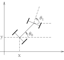
The applied transformation, consisting of a change of coordinates and feedback, is invertible, which proves that h = (x, y) are indeed flat outputs of the non-holonomic car. Still in Section 1.3, we illustrate our results by describing all flat outputs from some examples: non-holonomic car (1-trailer system) which we just discussed and then the n-trailer system.
Flatness of driftless two-input control systems
More generally, how to characterize all flat outputs of any 2-input driftless control system and how to describe their single loci and single controls. First, together with its proof, it will enable us to characterize all x-plane outputs of 2-input driftless systems (see Section 1.3).
Characterization of flat outputs
- Main Theorems
- Finding x-flat outputs
- Reducing equations for ϕ 2
- A complete description of x-flat outputs for the nonholonomic
- A complete description of x-flat outputs for the nonholonomic
It thus follows from Theorem 1.3.4 that for a given arbitrary ϕ1 (which satisfies the assumptions of the theorem), the choice of ϕ2 is unique in the sense that all functions ϕ2 giving x-planar outputs (ϕ1, ϕ2) actually yield statically equivalent x . - flat outputs. On the other hand, different choices of ϕ1 will lead to non-equivalent pairs of (ϕ1, ϕ2) x-plane outputs.
Proof of main theorems
- Useful results
- Proof of Theorem 1.2.2
- Proof of Theorem 1.3.2
- Proof of Theorem 1.3.3
- Proof of Theorem 1.3.4
In the above normal form, the integer m gives the number of singularities of the Kumpera-Ruiz normal form. This implies that the n-bar system is flat about any regular configuration and we show that the Cartesian position of the source point of the last (from above) bar is a flat output. As a by-product of our consideration, we deduce the global manageability of the n-bar system as it is accessible in any (regular or not) configuration.
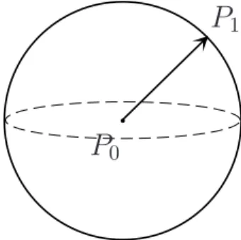
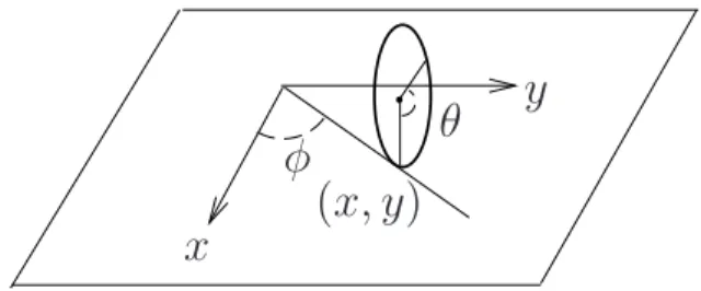
Model of a rigid bar moving in R 3
To obtain a kinematic model of the rigid bar, we need to restrict the ∆bar system to its true configuration space Q. To summarize, the model of the rigid bar system Γbar is defined by the ∆bar system, together with the holonomic constraint . The configuration space R3 ×S2 of the rigid bar system Γbar can also be naturally interpreted through classical rigid body theory.
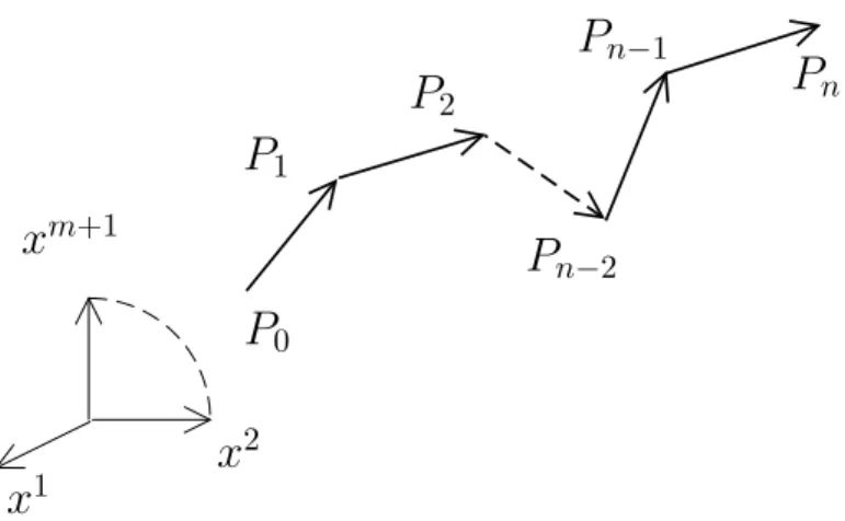
Model of the n-bar system moving in R m+1
It is now assumed that the instantaneous velocity of the point Pi is parallel to the vector. To obtain a kinematic model of the n-bar system we need to restrict the system ∆ to the regular submanifold Q ⊂ X. The presented model of the n-bar system in Rm+1 is a natural generalization of the well-known n-trailer. system on R2.
Equivalence of the n-bar system to the m-chained form
Another, albeit similar, model for the n-bar system (called the articulated arm) has been introduced and studied more recently in [71], and [72]; in the first a detailed singular locus analysis was performed (see also section 2.3.2). An alternative description of the above definitions can also be given using the dual language of differential forms. It turns out that alln-graphs are integral submanifolds of dimension 1, i.e. integral curves, of the Cartan distribution CCn(R,Rm).
Main result: equivalence of the n-bar system to the m-chained
Therefore, the statement that the control system Σ is locally inversely equivalent to the m-chain form (equivalent to the canonical contact system onJn(R,Rm)) will always mean that the associated distribution DΣ is locally equivalent to the Cartan distribution CCn( R,Rm ). The latter means in particular that the 2-bar system in R2 is transformable into a chain form, even if the two bars are rectangular. Of course, the 2-rod system in R2 is just a 1-trailer system (a unicycle-like mobile robot pulling a single trailer, or, equally, a non-holonomic car), and it is well known that the system can be brought into chain form even if the axes are perpendicular.
Proof of Theorem 2.3.3
- Notations
- Condition (i): D (n) = T Q
- Condition (ii) : D (n−1) contains a corank one involutive subdis-
- The regular locus of the n-bar system in R m+1
In other words, the rank 2 distributions on four-dimensional manifolds with the growth vector (2,3,4) have no singularities, a result going back to [11]. This shows that indeed every ω ∈ I(1) can always be expressed by a linear combination of the differential forms ω1, ω2,. Since Ln−1 and I both have constant rank, we immediately know that the relation Φ∗K⊥(q) ⊂ Φ∗J(q) holds if and only if.
Flatness of the n-bar system in R m+1
Any control u(t) ∈ The use of(x(t)) will be called singular and the trajectories of the system controlled by a singular control remain tangent to the characteristic distribution C1. The following theorem, given in [57], characterizes the minimal flat outputs for systems that are feedback equivalent to their chained form (i.e. the canonical contact system on Jn(R,Rm)), with m≥2. The following theorem describes the flatness property of then bar system Γ. 2) u0 is such that the instantaneous velocity P˙0 of the point P0 is non-zero (and therefore the instantaneous velocities P˙i, 0≤i≤n−1, are non-zero).
Proof of Lemma 2.4.1
It turns out that alln graphs are integral submanifolds, of dimension k, of a distribution called the Cartan distribution on Jn(Rk,Rm) and denoted by CCn(Rk,Rm). In the case of n = m = 1 and an arbitrary k, the solution is obtained by Darboux [10] in his famous theorem which generalizes previous results of Pfaff [55] and Frobenius [15]. In section 3.4 we recall Bryant's theorem (which describes the case n = 1, where k and m are arbitrary) and propose its extension which will be useful in proving our main result.
Cartan distributions for surfaces
So, in the case of constant rank, we can (locally) identify identity co-distributions and Pfaff systems, which is what we will do in this paper. In the paper, however, we will have to deal with non-smooth distributions D, in which q →dimD(q) jumps up at a point (and therefore is not lower semicontinuous). As we pointed out in the introduction, Jn(R2,Rm) can be fitted with a (non-integrable) distribution.
Characterization of Cartan distributions for surfaces
Main result
In Section 3.3.2, we will describe the relations of the Engel rank to the Cartan rank and, in particular, to the existence of involutive subdistributions of the corank k in D =I⊥. Second, it has an elegant geometric interpretation: it is equivalent to the existence of an involutive subdistribution, which we denote by Ln−1, of corank two in D(n−1). Given a distribution and a fixed point q∈M, condition (iv) can be checked algebraically because the involutive subdistribution Ln−1 is unique (if it exists) and computable; we will discuss it in section 3.3.2 below.
Involutive subdistributions of corank k
Extended Bryant normal form
Bryant normal form
Since m ≥ 3 and the Engel rank of D⊥ is equal to k, it follows by Theorem 3.3.4 that D contains an arbitrary subdistribution L that has cork k in D.
Extended Bryant normal form
Assume for a moment that ˜I satisfies the conditions of Theorem 3.4.2, then there is a local change of coordinates z = ψ(˜z) such that the collocation ψ∗I˜ is locally given in ˜z = (x, p)-coordinates, with Bryant's normal form (3.4.1). On the other hand, the condition rankEI = k implies that there is a 1-form Ω = Pm. remember that the coordinates are centered at zero). Let D be a distribution of constant rank k+mk+l, defined on the manifold M of dimension m+k+mk+l, so that D(1) =T M. If D satisfies, in the neighborhood of the point q∈M , the following conditions: . i) Engel's rank D⊥ is constant and equal to k,.
Proofs
Useful results
Furthermore, the condition that E is involutive and has constant cork r1+r2 implies that there exist r1+r2 smooth functions ϕ1,.
Proof of Theorem 3.3.2
Proof: (from Lemma 3.5.4) To explain the idea of the proof, we will show the lemma for k = 1 and then, after similar arguments, for any 1≤k ≤n. It is easy to see that the local diffeomorphism ϕ preserves the nested order of distributions.
Proof of Theorem 3.3.4
Note that the above system forms m relations obtained for 1≤i≤m with the corresponding differential forms ω1,. The above expression belongs to D⊥ (since fydωi ∈ D⊥) and therefore ηij(f) = 0 and πj(f) = 0, since the differential forms ηji, πj and ωs are independent. In [62], Respondek developed necessary and sufficient conditions for the orbital feedback linearization of a single-input system, which can be conveniently verified on the original system.
Orbital feedback equivalence
The system Σ defined by (4.2.1) is said to be orbital feedback linearizable if it is orbital feedback corresponding to a linear system of the form. Indeed, it is easy to observe that if Σ is orbital feedback corresponding to a time-increased linear system Λt via a negative time-rescaling function, it is via a positive time-rescaling function. To see it, suppose that Σ is orbital feedback corresponding to a time-augmented form (4.2.5) via a feedback transform and a time rescaling function given by γ <0.
Main result
The following generalization (OFL3) is needed to linearize the orbital feedback (see Lemma 4.6.1 in Section 4.6.1). Thus there exists a function φi for some 0≤i≤m such that Lfφi(x0)6= 0, where Lfφi denotes the Lie derivative of φi along the vector fieldf.
From distributions to control-affine systems and back
From distributions to control-affine systems
We note that the set of all admissible velocities of the control-affine system Σ atx ∈X is the affine subspace A(x) =f(x)+G(x) of the tangent space TxX. Therefore, to each control affine system there corresponds an affine distribution A = f +G, which assigns to each x ∈ X an affine subspace A(x) of TxX. Indeed, two control affine systems Σ and ˜Σ are inversely equivalent if and only if there exists a diffeomorphism ϕ such that.
From control-affine systems to distributions
Clearly, the function µ00 cannot be zero at x0 and β is invertible because the matrix M(x) is invertible everywhere. which implies that Σ is an orbital feedback equivalent to the canonical Brunovsky form with augmented t with a time-scale varying function γ =µ00. Σ is the orbital feedback equivalent to the t-augmented linear system Λt with all control indices equal to n+ 1. iii). The distribution DΣ associated with Σ satisfies the following conditions:. v) The distribution DΣ satisfies the following conditions, for 0≤j ≤n, (C1)′′ rank DΣ(j)= (j+1)m+1 and every element of DΣ(j) contains an involutive.
Examples
This illustrates an interesting phenomenon that the time rescaling linearization function is not unique and may lead to different control systems (in fact, Σ1, Σ2 and Σ3 are not mutually locally equivalent via a diffeomorphism φ in the state space) of which are, of course, equivalent reactions to each other. Consider a rigid bar moving at R3 so that the instantaneous velocity of the bar is parallel to its direction. As we explained in Remark 2 after Theorem 4.3.1, the choice of time rescaling function γ is not unique.
Proof of Theorem 4
Useful results
For simplicity, we can assume that the matrix B2 obtained by neglecting the first row of B is invertible, i.e. The following version of a result by Bryant [7] was given by Pasillas-L´epine and Respondek to study the Cartan distribution CCn(R,Rm). The condition (OFL1) assumes that the distributions Gfn+1 and Gfn are of constant rank and rankGfn+1−rankGfn=m. So if m≥3, by Lemma 4.6.3, the subdistribution B ⊂ Gfn given in point ( i) of Lemma 4.6.4 is involutive and unique.
Proof of Theorem 4.4.6
Dans le quatrième chapitre nous avons étudié le système de contrôle sous la forme Σ : ˙x=f(x)+Pm. Nous avons obtenu des conditions nécessaires et suffisantes vérifiables pour que le système linéarise Σ via une boucle orbitale. Est-il localement équivalent au système de contacts canonique sur Jn(R2,Rm).